Machine Learning and Real World Data

Lecture1

Sentiment classification — the task of automatically deciding whether a review is positive or negative, based on the text of the review

Lexicon – lexicon is a list of words with some associated information.

Suppose that a very large collection of documents describing the University of Cambridge has been collected. Your task is to build a classifier which assigns sentiment to each document, using the classes: positive, negative and neutral.

• Given the limited amount of annotated data, you decide to classify the documents using a standard sentiment lexicon. Explain how you would perform an experiment to do this.
  • Note that the preliminary description is important - we are told there is a large collection of documents, but we’re not told they are all of one genre. Unlike the artificially balanced sentiment data which was used for the practical, it is extremely unlikely the collection will be balanced - we might expect that the majority of the documents will be neutral.
    1. Tokenize the documents (will probably also require ‘cleaning’ by removal of markup)
    2. Classify the documents by counting matches with words in the sentiment lexicon (explain assumptions about sentiment lexicon and give details)
    3. It is necessary to establish some sort of threshold for positive/negative decisions: development data should be used to do this.
    4. Treatment of ties should be discusses (there are several reasonable options here)
    5. Adjustment for sentiment strength should be discussed (there are several reasonable options here)
    6. Split annotated data 50:50 into development set and final evaluation set.
    7. Note that some form of normalization for document length is required, but students are not expected to know this
• How would you evaluate the results of the system you have described in your answer to part (b) using the annotated data? Give details of the evaluation metrics you would use.
  • A decision has to be made as to how to use the annotated data for evaluation. The simplest method is to use majority class to decide on the gold standard. It is unlikely there will be many cases where the annotators have each chosen a different class, but such documents could be counted as neural.
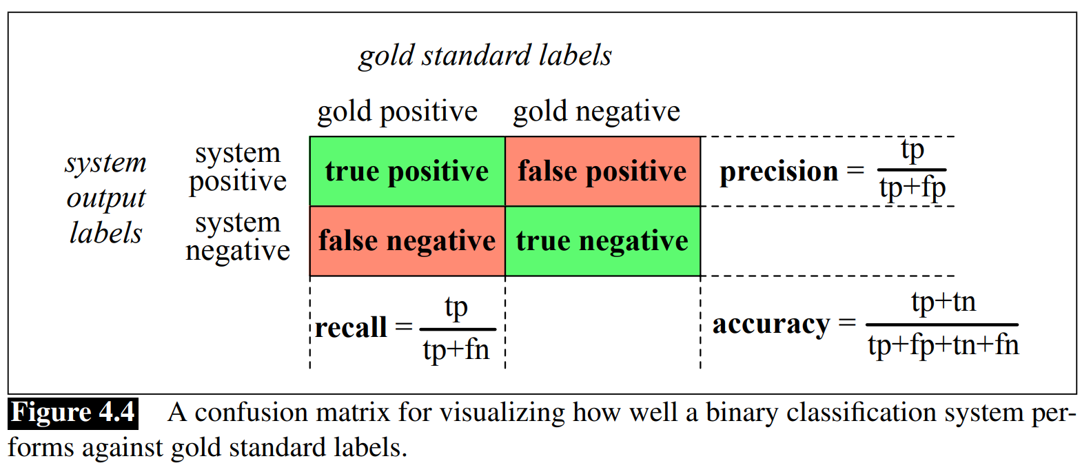
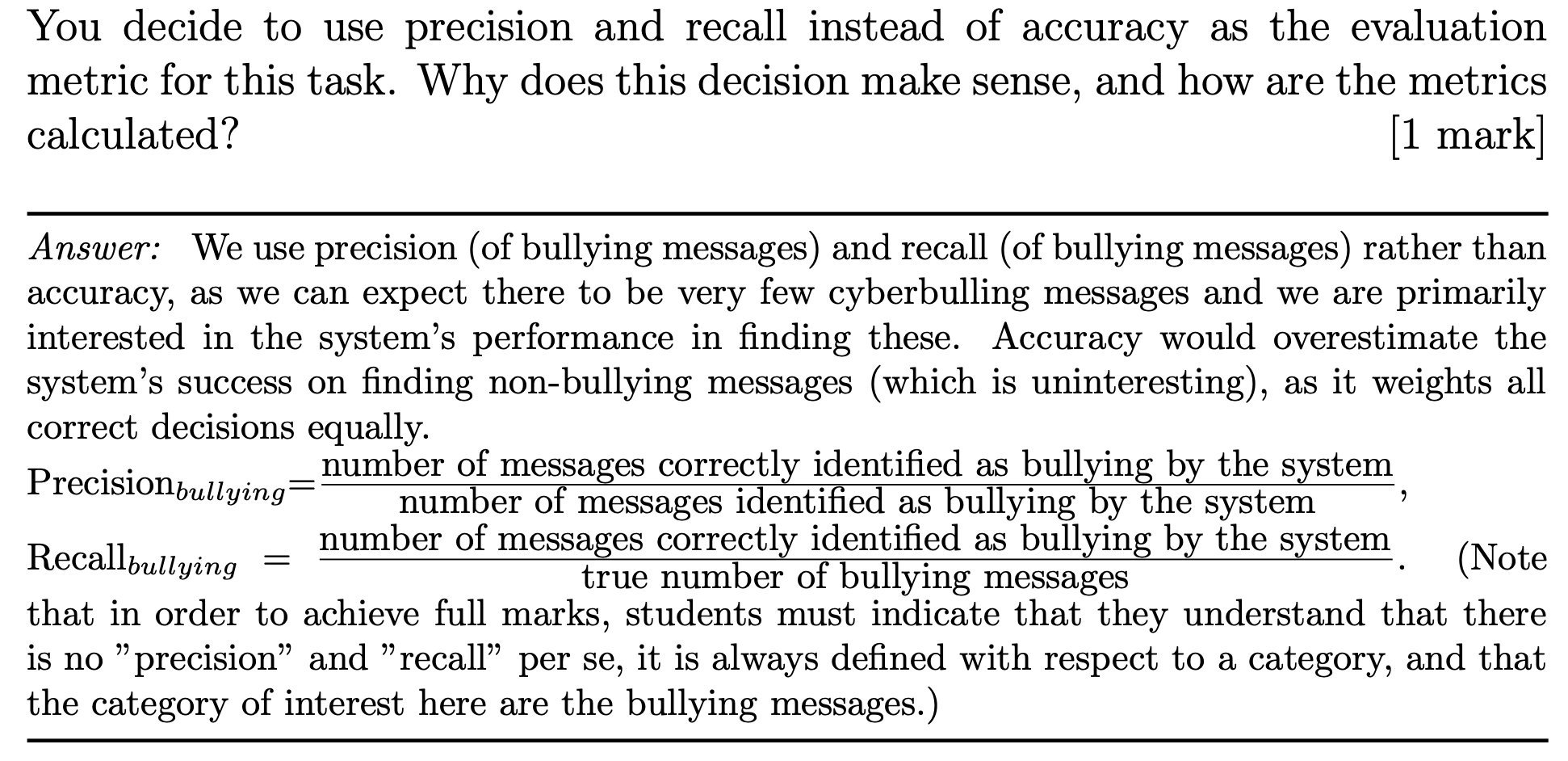
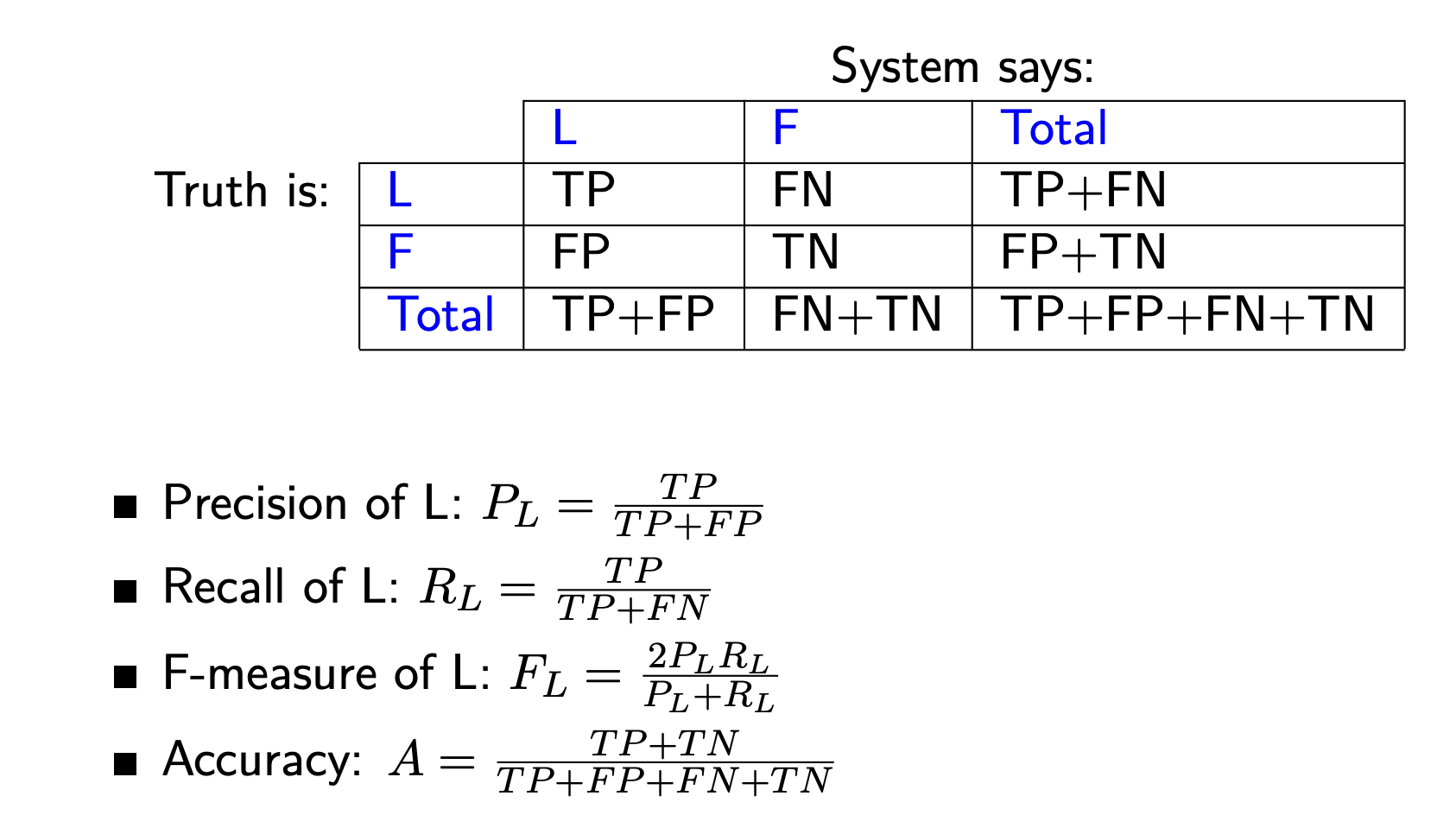
  • One can evaluate using precision and recall for each class. Accuracy will not work well because we cannot expect the dataset to be balanced
  • The alternative is to evaluate the system using kappa in conjunction with the human annotated data
• If the primary objective were to identify the documents with negative sentiment, how might your proposed evaluation change?
  • In this case, the distinction between the positive and neutral classes is unimportant. Recall should possibly be prioritized over precision on the negative class.
• It is suggested to you that the classes automatically assigned by the sentiment lexicon approach could be used to provide training data for a Naive Bayes classifier. Could such a classifier perform better than the sentiment lexicon classifier which provided the decisions it was trained on? Explain your answer
  • The Naive Bayes classifier could improve over the sentiment lexicon classifier in the circumstance where the sentiment lexicon was missing one or more words which were good cues for sentiment with this document set, assuming that such words did occur sufficiently often associated with words which were in the sentiment lexicon.
  • To see this, consider a toy example where the sentiment lexicon contains only the words good and bad. The document collection contains 1000 documents with both good and world-leading, 500 documents with only world-leading, 100 documents with only bad and 400 documents with none of these words. The test data has similar proportions: the first two sets are all both annotated as positive, the third set as negative and the fourth as neutral. Under these circumstances, the sentiment lexicon approach will classify the documents in the second set incorrectly, but the trained Naive Bayes algorithm would classify them as positive.
  • This amounts to using the sentiment lexicon as seeds for a semi-supervised classifier. There are more sophisticated approaches to this than simply using Naive Bayes on the automatically annotated data, but these have not been discussed in the course so it is not expected that the answer includes details of such an approach

Type vs. Token

In natural language processing (NLP), a "type" refers to a distinct word or symbol in a language, while a "token" refers to a specific instance of that word or symbol in a text. For example, in the sentence “the cat in the hat,” the word “the” is a type, but it appears twice as two different tokens in the sentence. This distinction is important because it allows for the calculation of various statistics in NLP, such as the type-token ratio.

• Any unique word is a type. Any given instance of a type is a token.

Provide a sentence with exactly 4 types and 5 tokens. Explain any assumptions you make about the nature of tokens.

Any 5 word sentence that contains one word type twice: e.g. the cat likes the dog In this example we assume that punctuation is removed and that all word tokens are lowercased. If this wasn’t the case we could have a sentence like A long long winding road. (1 mark for sentence, 1 mark for discussion of tokens)

Lecture2: Naive Bayes

What is machine learning?

• A program that learns from data
• A program that adapts after having been exposed to new data.
• A program that learns implicitly from data.
• The ability to learn from data without explicit programming.

Terminology

Features are easily observable (and not necessarily obviously meaningful) properties of the data.

Classes are the meaningful labels associated with the data.

Classification then is function that maps from features to a target class.

Probabilistic classifiers provide a distribution over classes

• Given a set of input features, a probabilistic classifier returns the probability of each class.
• That is, for a set of observed features $O$ and classes $c_1, \ldots, c_n \in C$, it gives $P(c_i|O)$ for all $c_i \in C$.
• For us, $O$ is the set of all the words in a review ${w_1, w_2, \ldots, w_n}$ where $w_i$ is the $i$th word in a review, and $C = {\text{POS}, \text{NEG}}$
• We get: $P(\text{POS}|w_1, w_2, \ldots, w_n)$ and $P(\text{NEG}|w_1, w_2, \ldots, w_n)$.
• We can decide on a single class by choosing the one with the highest probability given the features:

$$
\hat{c} = \arg\max_{c \in C} P(c|O)
$$

(multinomial) Naïve Bayes classifier

Bag of words: an unordered set of words with their position ignored, keeping only their frequency in the document

• Naïve Bayes classifiers are simple probabilistic classifiers based on applying Bayes’ theorem.

Bayes Theorem

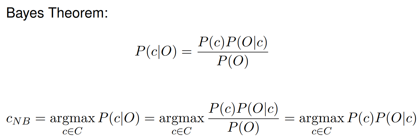
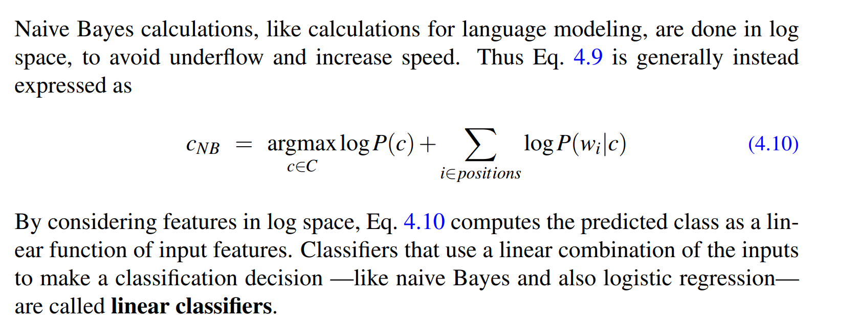
• We can remove P(O) because it will be constant during a given classification and not affect the result of argmax
• $P(c)$: prior probability; $P(O|c)$: likelihood
• We call Naive Bayes a generative model because we can read the above equation as stating a kind of implicit assumption about how a document is generated:
  1. A class is sampled from $P(c)$
  2. Words are generated by sampling from $P(O|c)$

Naive Bayes theorem

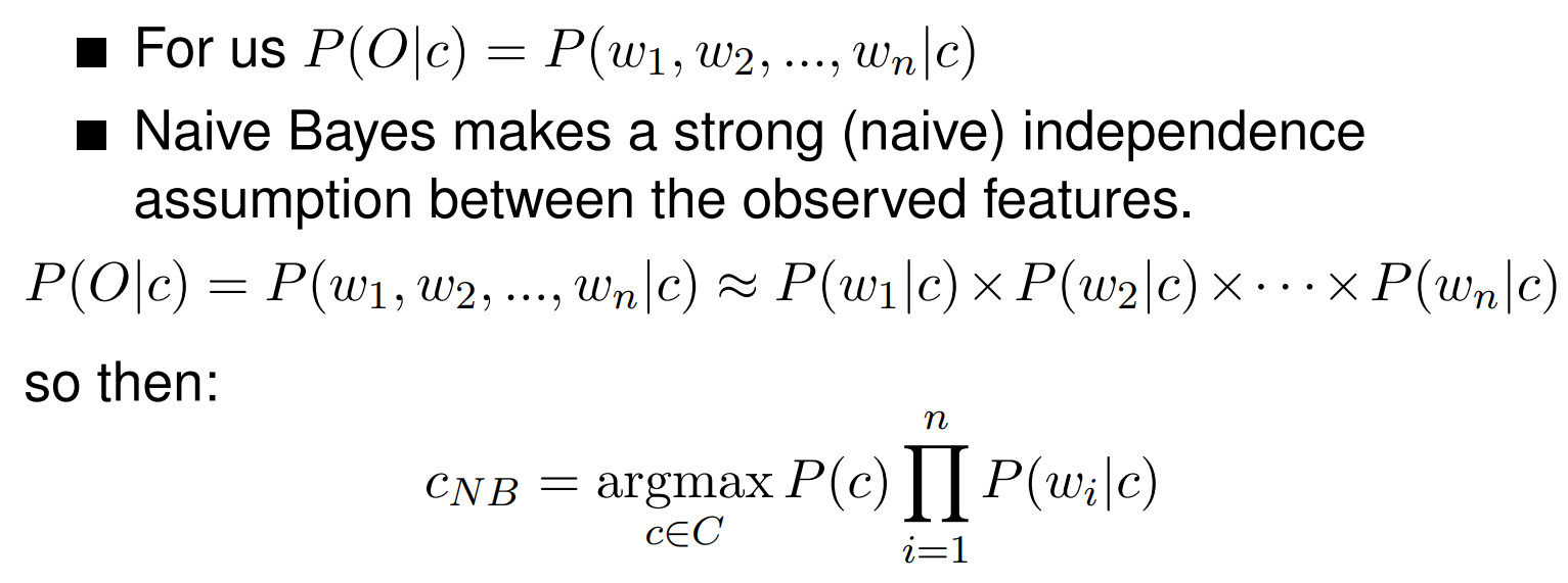
• The position of the words in ignored and we make use of frequency of each word

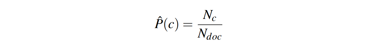
Estimate for paramters of Naive Bayes

• $P(C)$

• $P(f_i|C)$

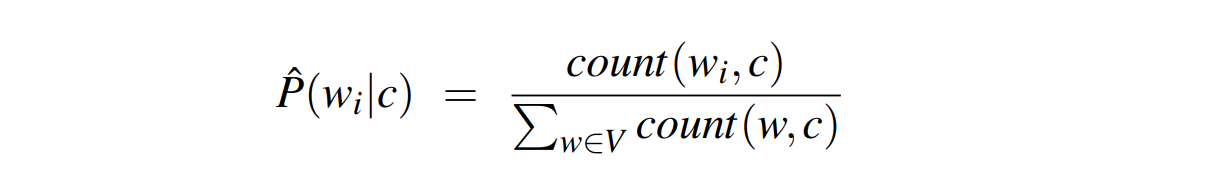
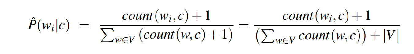
Here the vocabulary $V$ consists of the union of all the word types in all classes, not just the words in one class $c$.

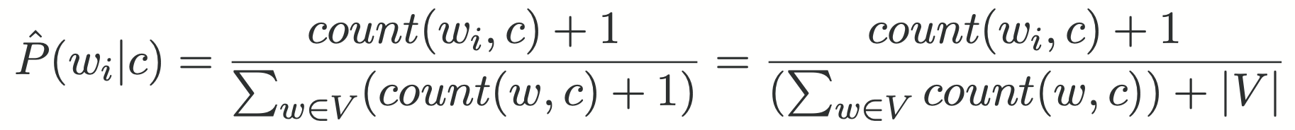
Laplace smoothing

Calculations

Full algorithm

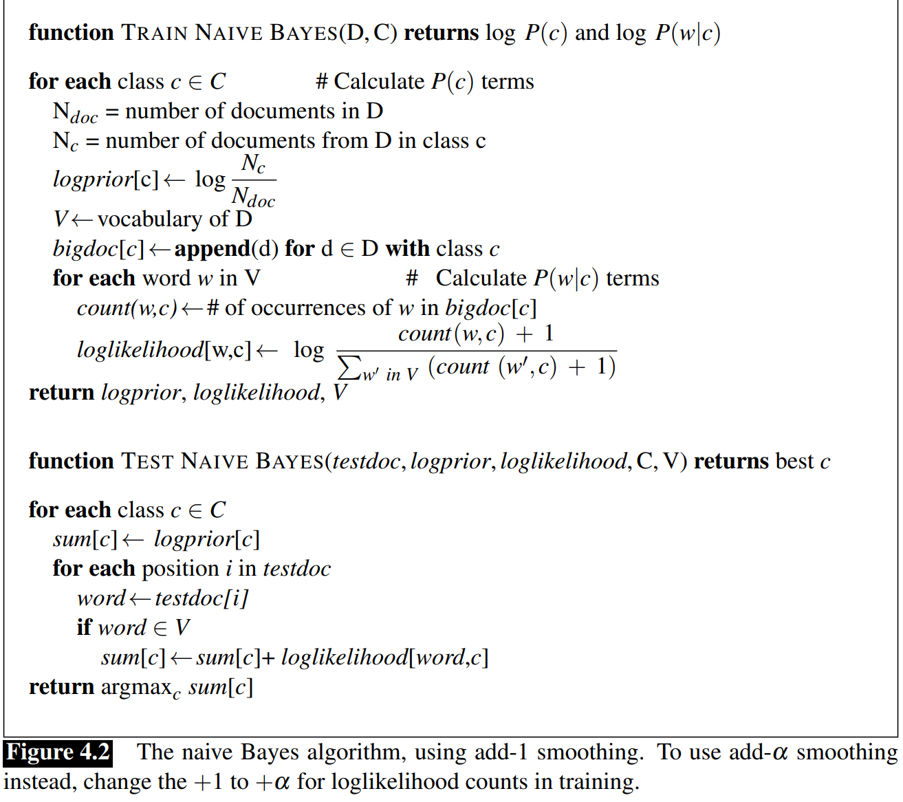
function Train Naive Bayes(D,C) returns log P(c) and log P(w|c)
  for each class c in C: #Calculate P(c) temrs
    N_doc = number of documents in D
    N_c = number of documents from D in class c
    logprior[c] = log(N_c/N_doc)
    V = vocabulary of D
    bigdoc[c].append(d) for d in D with class c
    for each word in V: #calculate P(w|c) terms
      count(w,c) = # of occurance of w in bigdoc[c] 
      loglikelihood[w,c] = log((count(w,c)+1)/sum(count(w`,c)+1 for w in V))
  return logprior, loglikelihood, V

function Test Naive Bayes(testdoc, logprior, loglikelihood, C, V) returns best c
	for each class c in C:
    sum[c] = logprior[c]
    for each position i in testdoc:
      word = testdoc[i]
      sum[c] += loglikelihood[word,c]
  return argmax_c sum[c]

2018-p03-q07

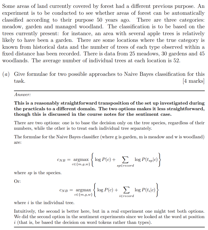
How could you derive parameter estimates for use in the Naive Bayes classifiers from this type of data?

We need to calculate the probabilities $P(g)$, $P(m)$, $P(w)$, which is relatively straightforward.

Additionally, we need to calculate conditional probabilities such as

$P(\text|g)$ or $P(\textNaN|g)$.

In the first option, we count each species only once for each record. The probability is then calculated as the number of records for the category where the species appears, divided by the total number of records for the category:

$$ P(\text|g) = \frac{\text{count(records with species in category g)}}{\text{count(all records in category g)}}$$

For the second option, we calculate the number of individual trees of each species, divided by the total number of individual trees in that category:

$$ P(\text{tree-of-species}|g) = \frac{\text{count(trees of species in category g)}}{\text{count(all trees in category g)}} $$

Both probabilities need to be smoothed to avoid zero probabilities. In the practicals, we have used add-one smoothing, where 1 is added to every count, including the zero counts. Thus, the smoothed probabilities become:

$$ P(\text{species}|g)_{\text{smoothed}} = \frac{\text{count(records with species in category g)} + 1}{\text{count(all records in category g)} + N} $$

$$ P(\text{tree-of-species}|g)_{\text{smoothed}} = \frac{\text{count(trees of species in category g)} + 1}{\text{count(all trees in category g)} + N} $$

where N is the number of distinct species (or tree-of-species, depending on context).

How could you used the available data to train and test a Naive Bayes classifier?

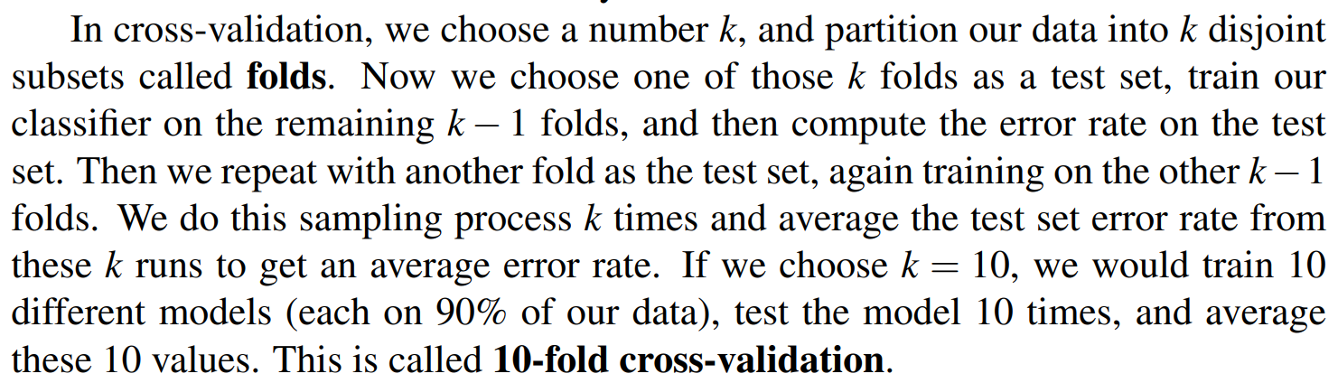
Given the limited number of data points, it is essential to use cross validation. i.e., the data should be split into folds, with a different fold held out for testing each time. Since the split between the categories is uneven, it would be reasonable to use stratified cross-validation (i.e., balance the categories in each fold). The amount of data is too small for 10-fold cross validation: 5-fold is more reasonable. The mean accuracy and variance across the folds should be reported.

Although we have suggested that there should always be some completely unseen data for final evaluation, there really isn’t enough data to make this possible.

The cross-validation experiment should ideally be repeated with different data splits.

Accuracy alone is not fully informative. Ideally one wants to report the confusion matrix, although the practicals do not go into the details of methodology with multiple classes so this is a bonus point rather than part of the expected answer.

You are now given a large catalogue of tree species with each species manually assigned to zero or more of the categories. Describe a modification to your previous experiment which makes use of this data.

Given that there might be some data sparsity (which is likely due to the relatively small amount of data), the best way to utilize the additional data would probably be to enhance the smoothing. Assuming that we’ve previously described add-one smoothing, a simple approach would be to parameterize the smoothing based on whether the tree species was associated with the category in the list.

For instance, if there are no cases of apple trees in meadows in the collected data, and the apple tree is not listed under meadow in the catalogue, the smoothing parameter might be set to 0.1. Conversely, if the tree species is associated with the category, a smoothing parameter of 1 could be used.

An alternative approach would be to use the additional data to improve the classification in cases where the Naive Bayes (NB) classifier was not making a clear decision. The challenge with this approach is that the probability estimates from the NB classifier are unlikely to be very accurate.

Regardless, this experiment would involve some parameters (like the 0.1 vs 1 for smoothing) that need to be tuned. The course notes have mentioned this process of tuning parameters.

Demonstrating improvement would be challenging without additional data, unless the difference between methods is substantial. Conducting a proper significance test would essentially be impossible due to the lack of data.

Training and Testing

Training: the process of making observations about some known data set

In supervised machine learning you use the classes that come with the data in the training phase

Testing: the process of applying the knowledge obtained in the training stage to some new, unseen data

==We never test on data that we trained a system on==

• Make sure the ratio of the classes is the same for both, particular the case for unbalanced classes
• We shouldn’t test of the same data more than once

train:dev:test

In the dev set, we allow ourselves to repeat on this set. (Used for hyper-parameter tuning)

The problem is what we called overfitting:

• A machine learning model performing exceedingly well on the training data but failing to generalize accurately to unseen data.

Unknown words (ignore!)

Stop words (ignore!)

Optimizing for Sentiment Analysis

Binary multinomial Naive Bayes

• For sentiment classification and a number of other text classification tasks, whether a word occurs or not seems to matter more than its frequency. Thus it often improves performance to clip the word counts in each document at 1.

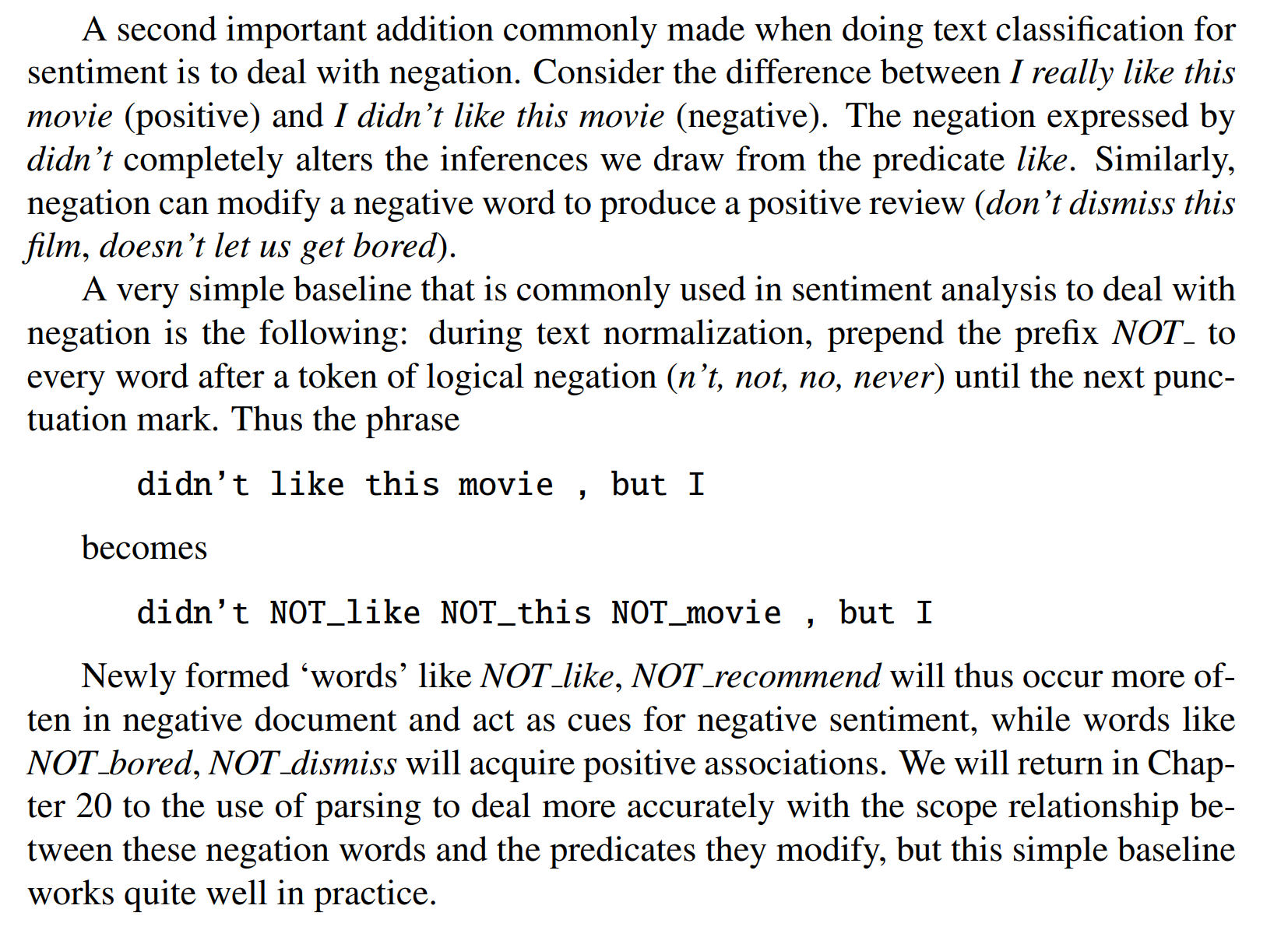
Deal with negation

Lexicon-based information

How can you use lexicon-based information to make your classifier more robust towards languages change?

The key to this question is that the NB classifier needs to be regularly retrained, and that we need a cheap way of finding new informative training material. The lexicon can help in this. We could run a lexicon-based approach on some new training data sourced from the incoming message stream.

An alternative method is to use the labels predicted by the current NB system as training material for the next NB retraining. This might help if new words occur sufficiently often in a message together with those from the lexicon

You could also go down an Active learning route by trying to find the training examples most likely to be informative, and have a human annotate those for retraining the NB classifier.

Voting between classifiers.

Evaluation: precision, recall, F-measure

2021-p03-q09

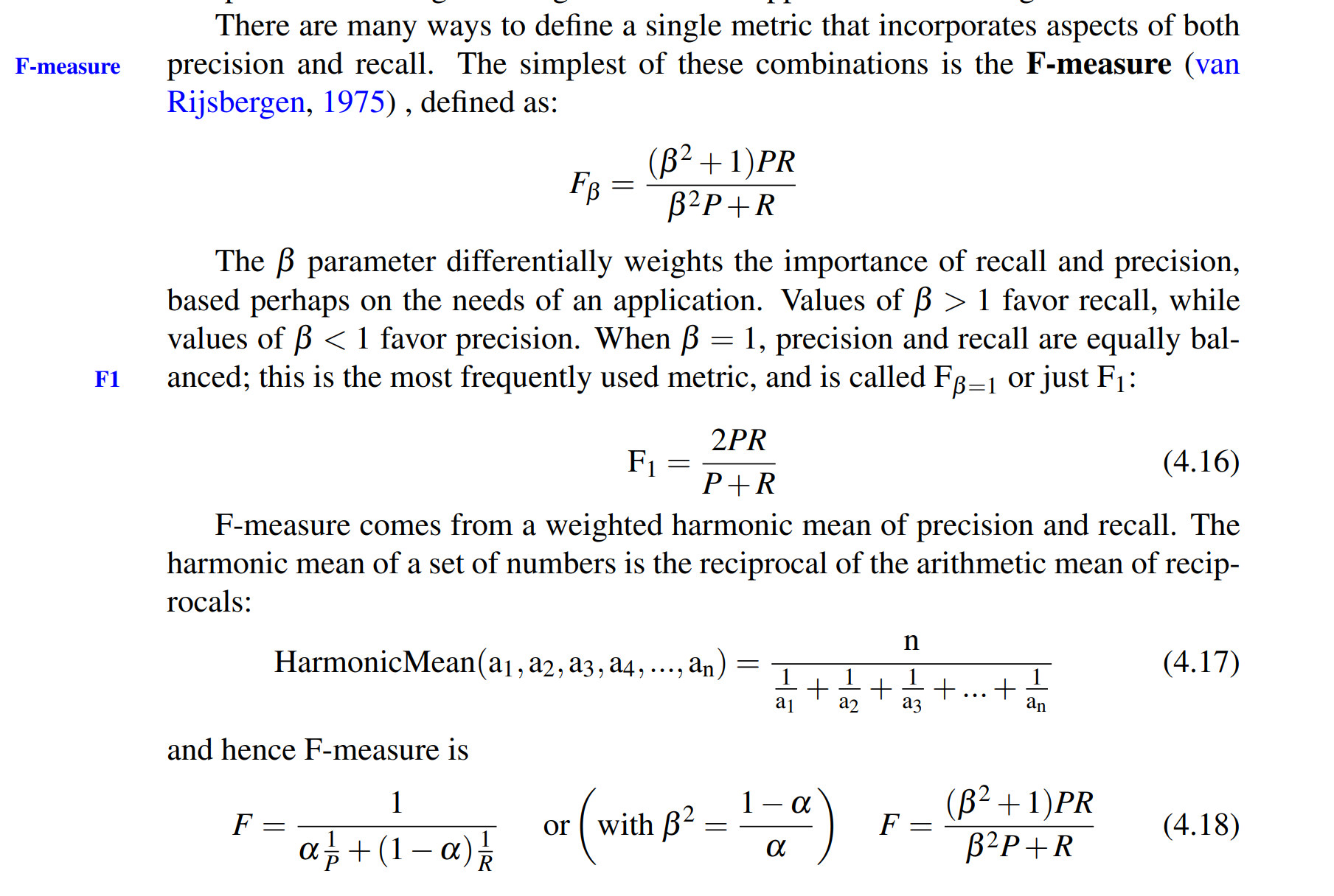
F-measure

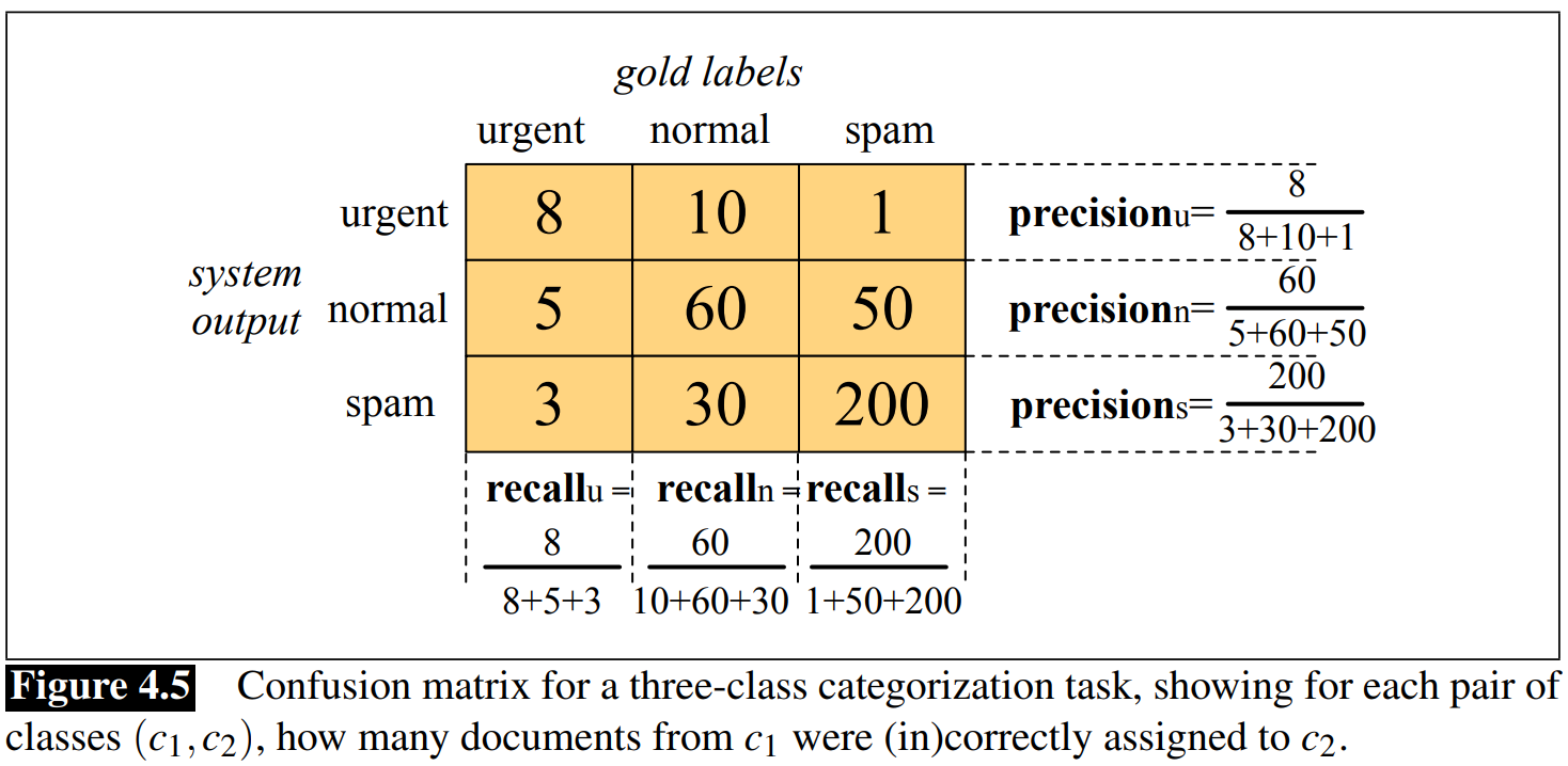
Evaluating with more than 2 classes

Cross Validation

Past papers

2020-p03-q07

2021-p03-q09

Lecture3: Zipf’s Law and Heap’s Law

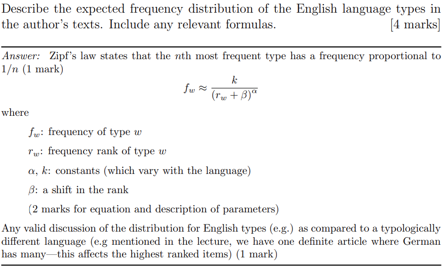
Zipf’s law

Word frequency distributions obey a power law

• There are a large number of high frequency words
• There are a small number of low frequency words

The nth most frequent word has a frequency proportional to 1/n
$$
f_w \approx \frac{k}{r_w^a}
$$
$f_w$: frequency of word $w$

$r_w$: frequency rank of word $w$

$\alpha,k$: constants, which may vary with the language

• e.g. $\alpha$ is around 1 for English but 1.3 for German

Actually
$$
f_w \approx \frac{k}{(r_w+\beta)^\alpha}
$$
$\beta$: a shift in the rank

Other examples

• Sizes of settlements
• Frequency of access to web pages
• Size of earthquakes
• Word senses per word
• Notes in musical performance
• Machine instructions

Zipf curves in log-space

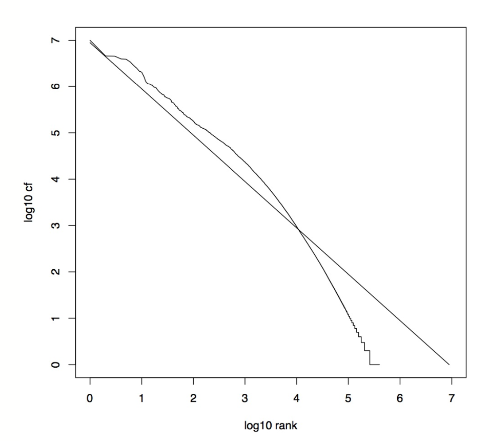
By fitting a simple line to the data in log-space we can estimate the language specific parameters α and k

Heap’s law

• We call any unique word a type: “the” is a word type
• We call an instance of a type a token: there are 13721 “the” token in Moby Dick

Describes the relationship between the size of a vocabulary and the size of text that give rise to it

$$
u_n = kn^\beta
$$

where

$u_n$: number of types (unique items) i.e. vocabulary size

$n$: total number of tokens i.e. text size

$\beta, k$: constants (language dependent)

• $\beta$ is around $\frac{1}{2}$
• $30 \le k \le 100$

Zipf’s law and Heaps’ law affected our classifier

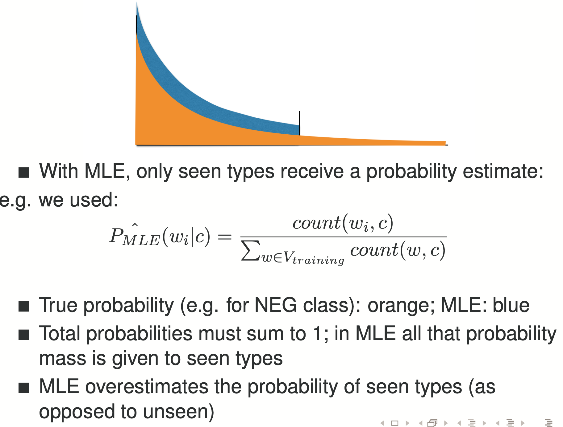
Smoothing redistribute the probability mass

• It takes some portion away from MLE estimation
• It redistribute this portion to unseen types
• Better estimate; still not perfect

Lecture 4

Specificity and Power of a Test

When performing a significance testing: there are two things we don’t want it to happen:

• That a test declares a difference when it doesn’t exist (Type 1 error)
  • $\alpha$ is the probability that this happens
  • $1-\alpha$ is called the specificity of a test
  • Specificity issues
    • This should never happen (problem of scientific ethics)
    • Develop an intuition when numbers look “too good to be true”
    • You probably used the wrong test (which has built in assumptions that won’t apply)
• That a test declares no difference when it does (Type 2 error)
  • $\beta$ is the probability that this happens
  • $1-\beta$ is called the power of a test
  • Power issues
    • This is quite common
    • Use a more powerful test, for example permutation test rather than sign test
    • Use more data
    • Change your system so there’s a stronger effect
    • Hopefully your $p$ will decrease and finally reach below $\alpha$

Significance Reporting - the three deadly sins

• Case 1: No significance test performed, statements of “better” and “outperform” and the like are used only based on raw comparisons of numbers → Methodological Unsoundness

• Case 2: Significance test was performed, but statements of “better” etc are still made for all differences, even the insignificant ones → Scientific illiteracy

• Case 3: No test are performed, statements of “better” etc are made just on basis of raw differences, and the keyword “significant“ is still used, often to refer to big effect sizes → Scientific fraud

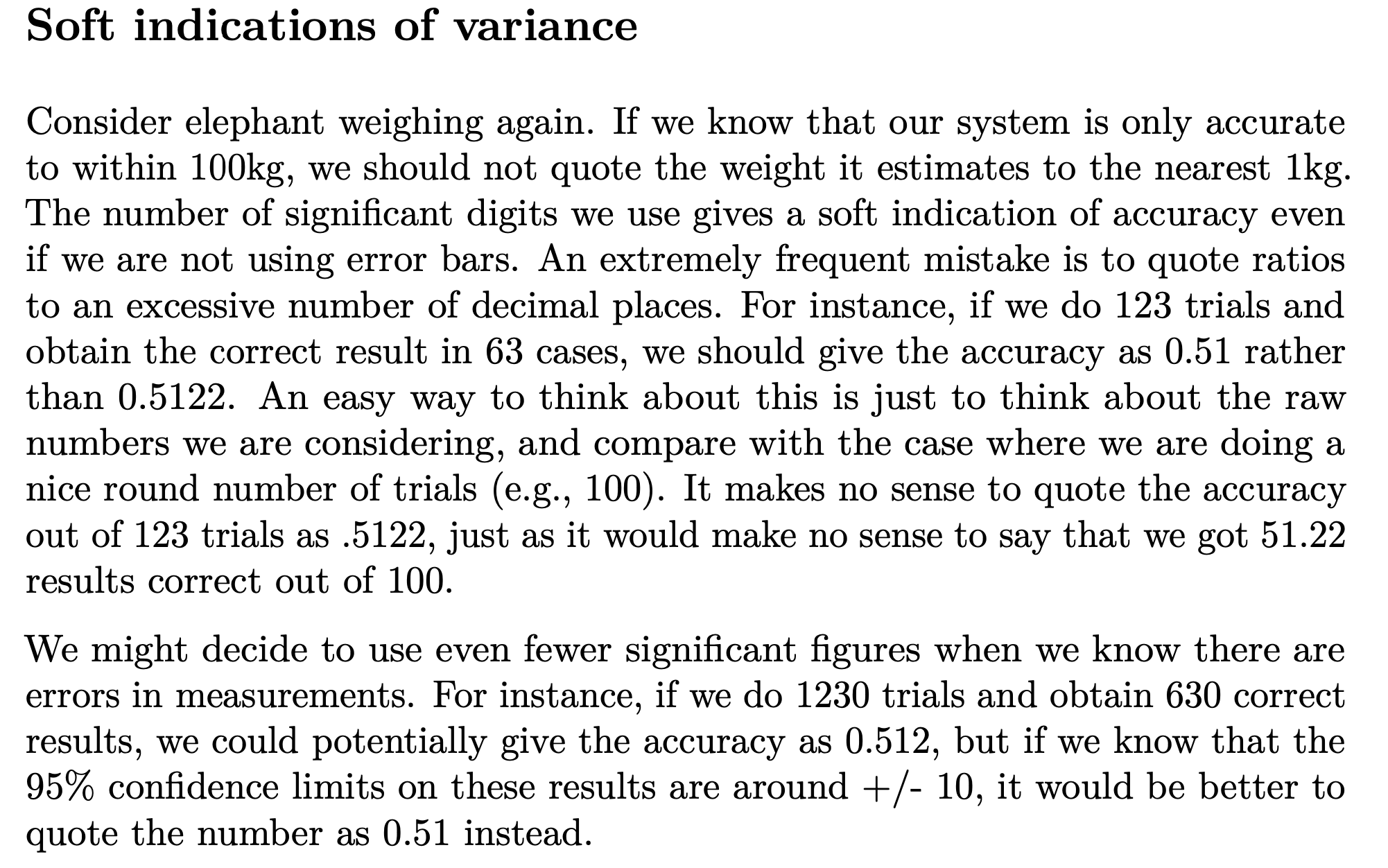
Significant Digits

• For instance, when deciding whether you should report 0.34 or 0.344, you should only report three digits if the difference between 0.340 and 0.344 is likely to be significant on your dataset

Trouble shooting

• Getting accuracies per each class can sometimes point out problems

Significance testing

---

Past papers

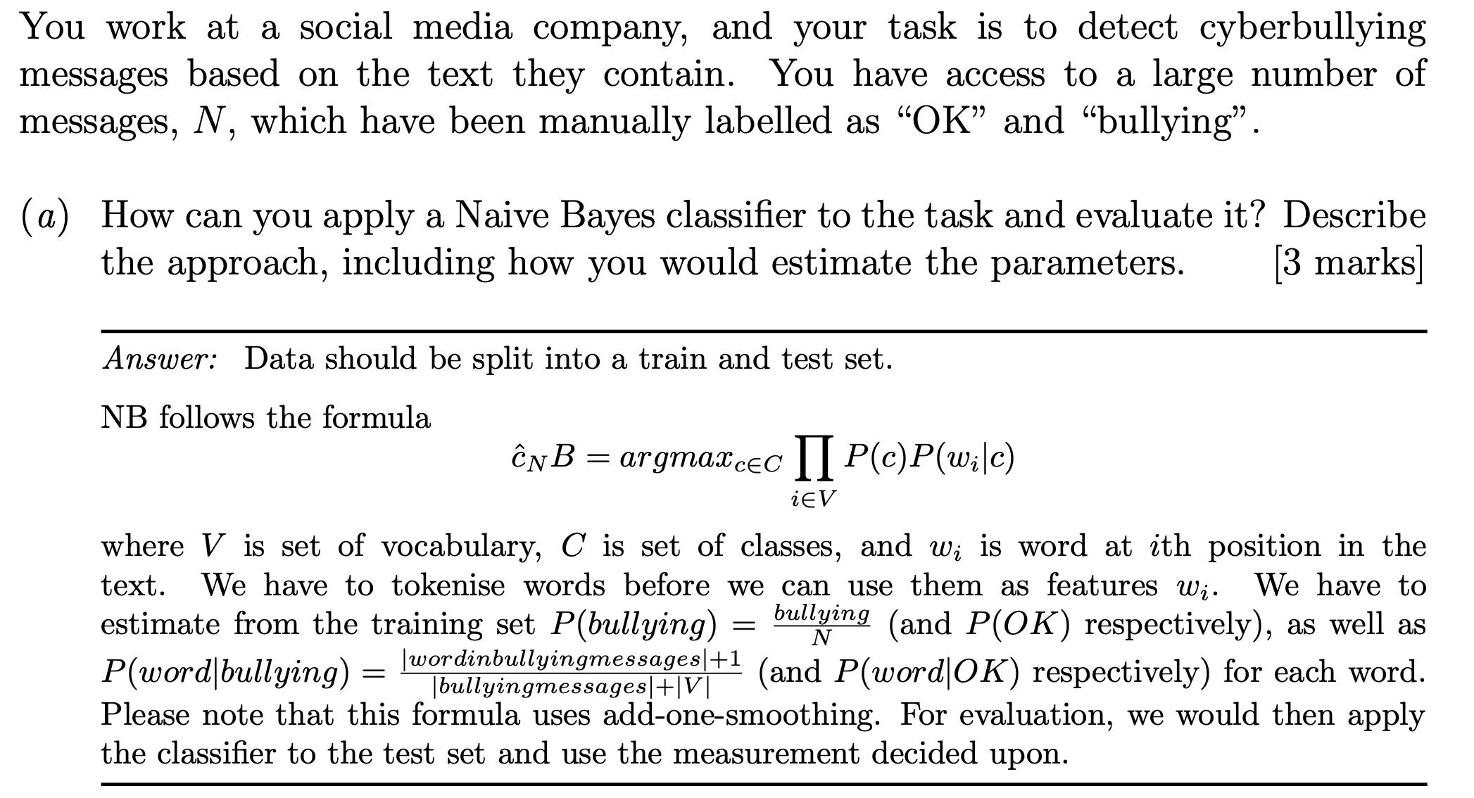
A piece of writing has been discovered which both of our authors claim to design be theirs. Could the classifier be used to settle this authorship dispute? Explain your answer.

Accuracy of the classifier may be measured on a test set that was not used during training or development of the classifier (1 mark). Accuracy is the number of correct decisions divided by total decisions (1 mark). Could test the significance of the result against a baseline system that selects between the 2 classes at random—null hypothesis being that your classifier is only as good as uniform chance (1 mark) The classifier could not prove authorship but can give a probability of the author given the training data (1 mark).

Lecture5

Ability to generalise

• We want a classifier that performs well on new, never-before seen data.

• That is equivalent to saying we want our classifier to ==generalise== well.

• We want it to:

  • Recognise only those characteristics of the data that are general enough to also apply to some unseen data
  • Ignore the characteristics of the training data that are specific to the training data

Because of this, we never test on our training data, but use separate test data. But overtraining can still happen even if we use separate test data.

Overtraining/Overfitting/Type III errors

• Overtraining is when you think you are making improvements (because your performance on the test data goes up)

• but in reality you are making your classifier worse because it generalises less well to data other than your test data.

• You could make repeated improvements to your classifier, choose the one that performs best on the test data, and declare that as your final result.

• By repeatedly using the test data, you have lost the effect of it being surprising, really unseen data.

• The classifier has now indirectly also picked up accidental properties of the (small) test data.

Overtraining, the hidden danger

• You have to actively work harder (be vigilant) in order to notice that it is happening
• But you may be tempted not to notice it

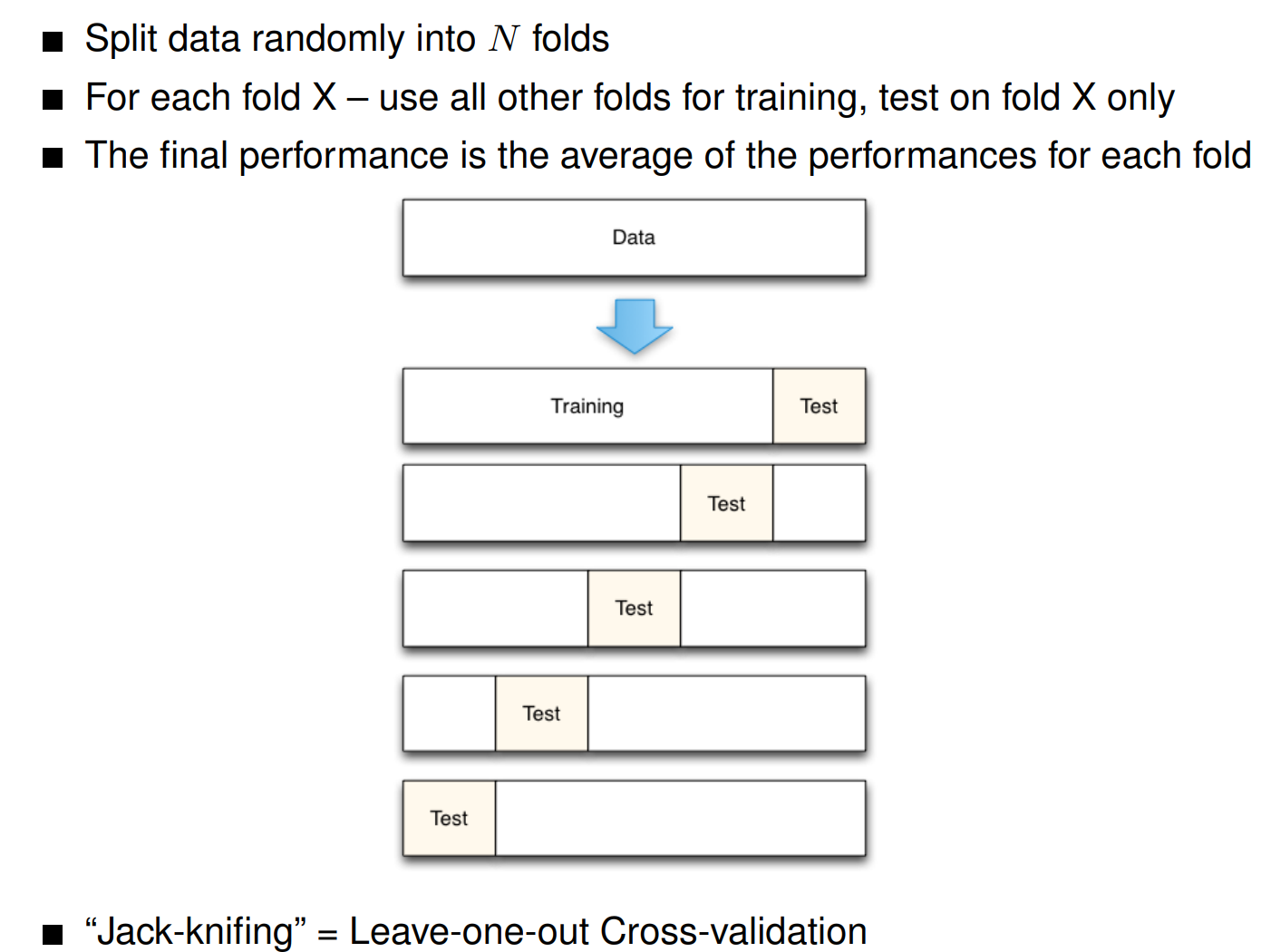
N-Fold cross-validation

Motivation

• We can’t afford getting new test data each time.
• We must never test on the training set.
• We also want to use as much training material as possible (because ML systems trained on more data are almost always better).
• We can achieve this by using every little bit of training data for testing – under the right kind of conditions.
• By cleverly iterating the test and training split around.

仍然有分training, dev, 和 test. test最后用. 图中的test set是dev set的意思.

Variance between splits

• If all splits performed equally well, this is a good sign

$$
var = \frac{1}{n}\sum\limits^n_i(x_i-\mu)^2
$$

• $x_i$: the score of the $i^{th}$ fold
• $\mu$: $avg(x_i)$: the average of the score

Stratified cross-validation

A special case of cross-validation where each split is done in such a way that it mirrors the distribution of classes observed in the overall data.

Cross-validation doesn’t solve all our problems

• Cross-validation gives us some safety from overtraining.
• Nevertheless, even with cross-validation, we still use data that is in some sense “seen.”
• So it is no good for incremental, small improvements reached via feature engineering.
• We also cannot use the cross-validation trick to set global parameters because we only want to accept parameters that are independent of any training.
• As always, the danger is learning accidental properties that don’t generalize.
• Enter the validation corpus.

Validation Corpus

• The validation corpus is never used in training or testing.
• We can therefore use this corpus for two useful purposes:
  • We can use it to set any parameters in any algorithm before we start with training/testing.
  • We can also use this corpus as a stopping criterion for feature engineering.
    • We can detect “improvements” that help in cross-validation over the train corpus but lead to performance losses on the validation corpus.
    • We stop “fiddling” with the features when the result on the validation corpus starts decreasing (in comparison to the cross-validation results).
    • Then, and only then, do we measure on the test corpus (once).

Lecture 6 Agreements

So far, your datasets have contained only the clearly positive or negative reviews

• Only reviews with extreme star-rating were used.
• This is a clear simplification of the real task.
• If we consider the middle range of star-ratings, things gets more uncertain.

Human agreement

Human agreement is the only empirically available source of truth in decisions which are influenced by subjective judgement.

• Something is true if several humans agree on their judgement, independently from each other
• The more they agree the more true it is

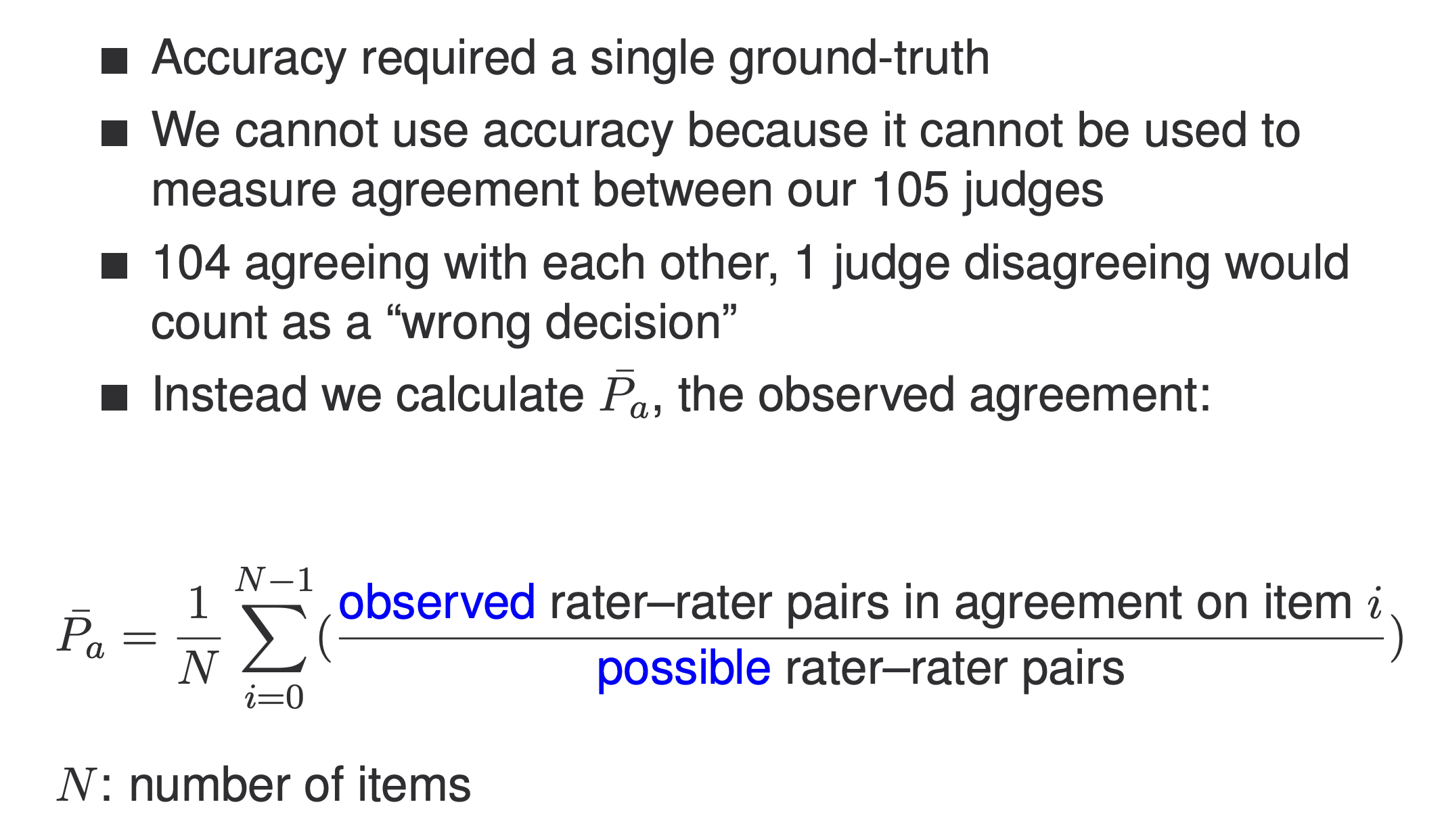
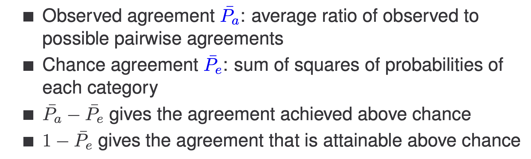
Observed Agreement

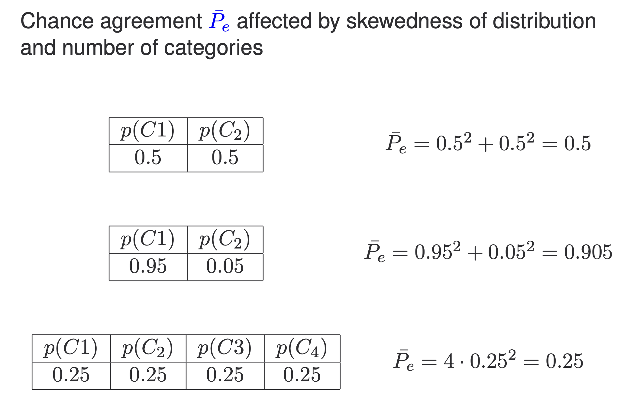
Chance agreement

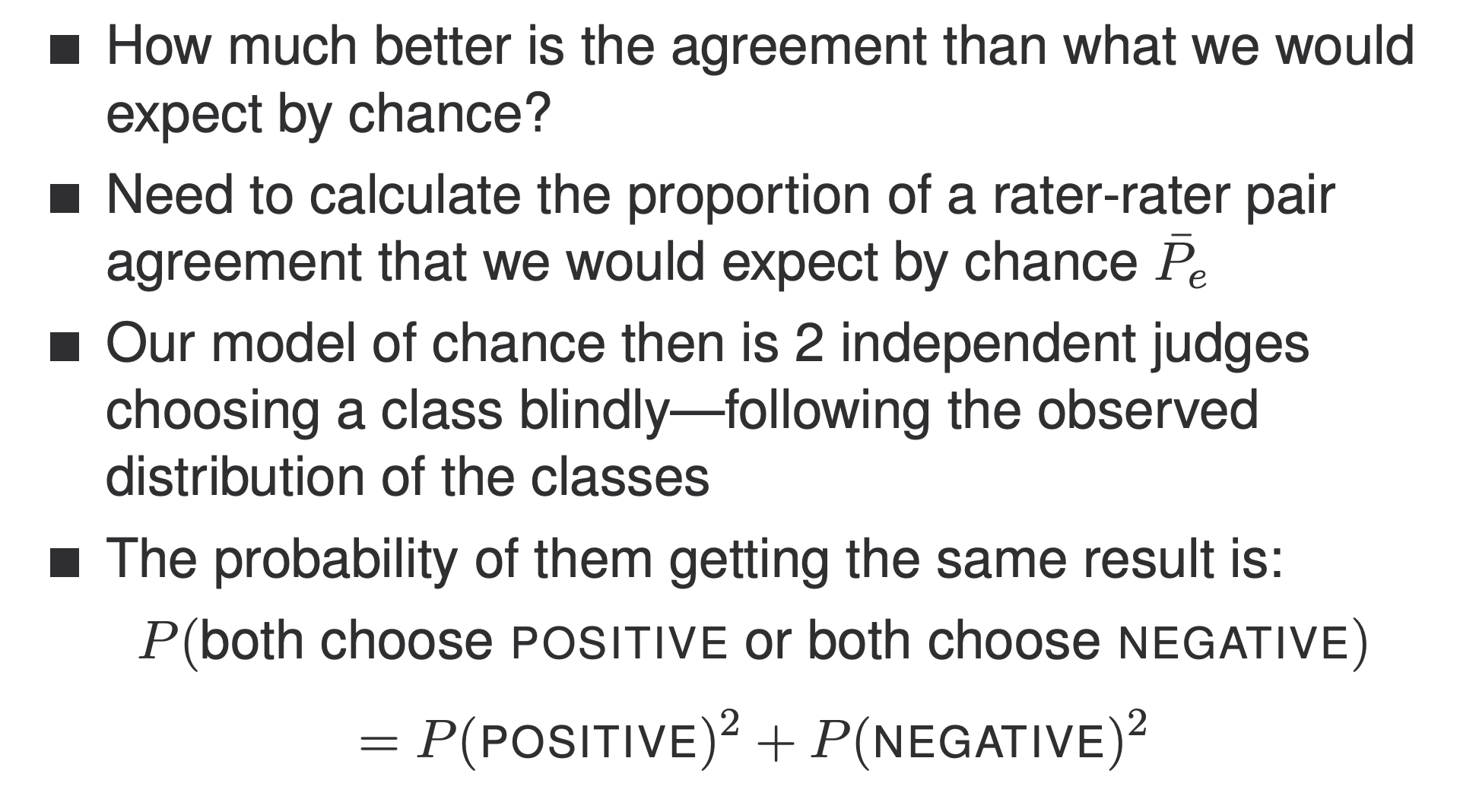
Reliability of agreement: Fleiss’ Kappa

• Measures the reliability of agreement between a fixed number of raters when assigning categorical ratings
• Calculates the degree of agreement over that which would be expected by chance

$$
k = \frac{\bar{P}_a-\bar{P}_e}{1-\bar{P}_e}
$$

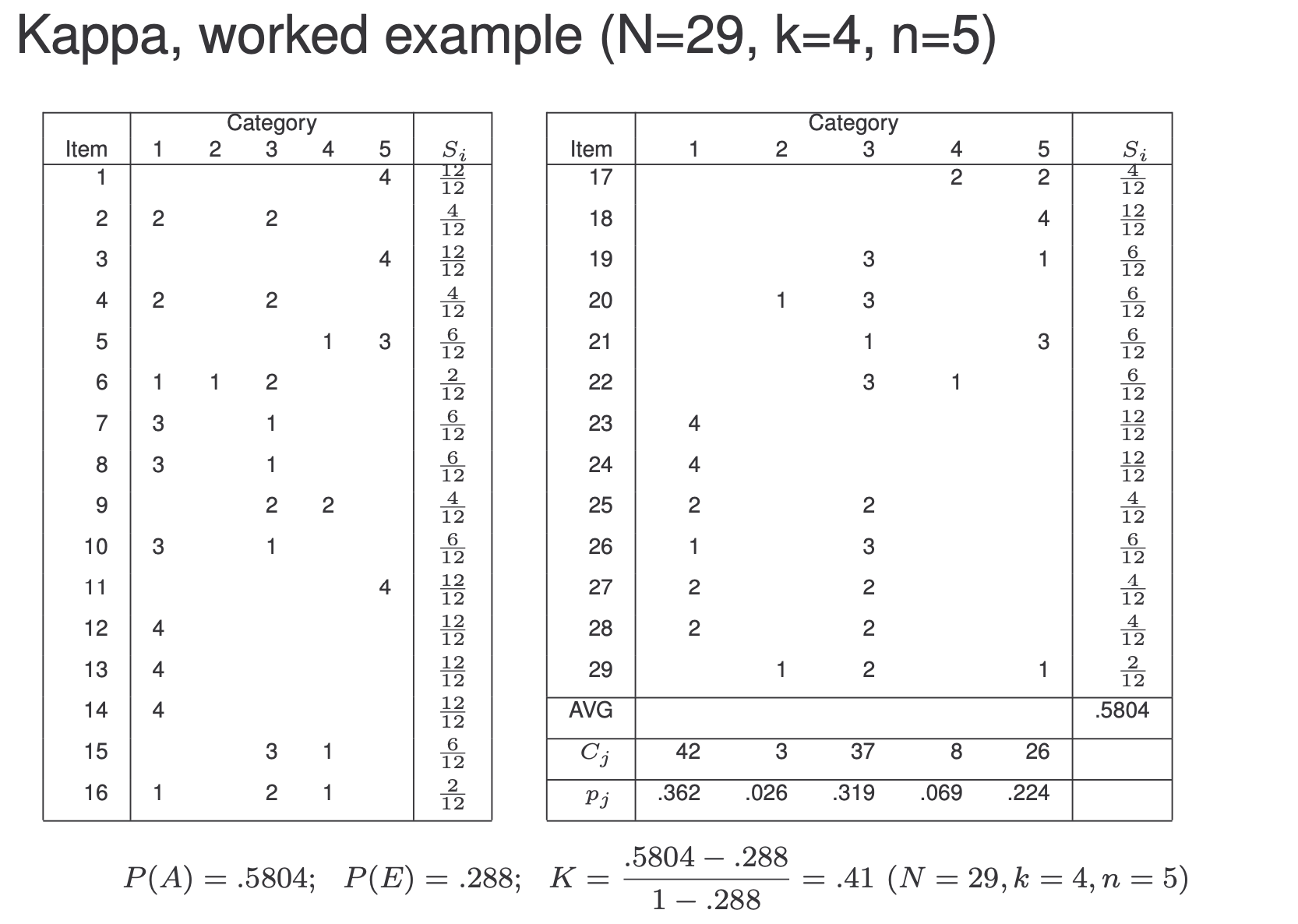
$N$: number of items

$k$: number of judges

$n$: number of categories

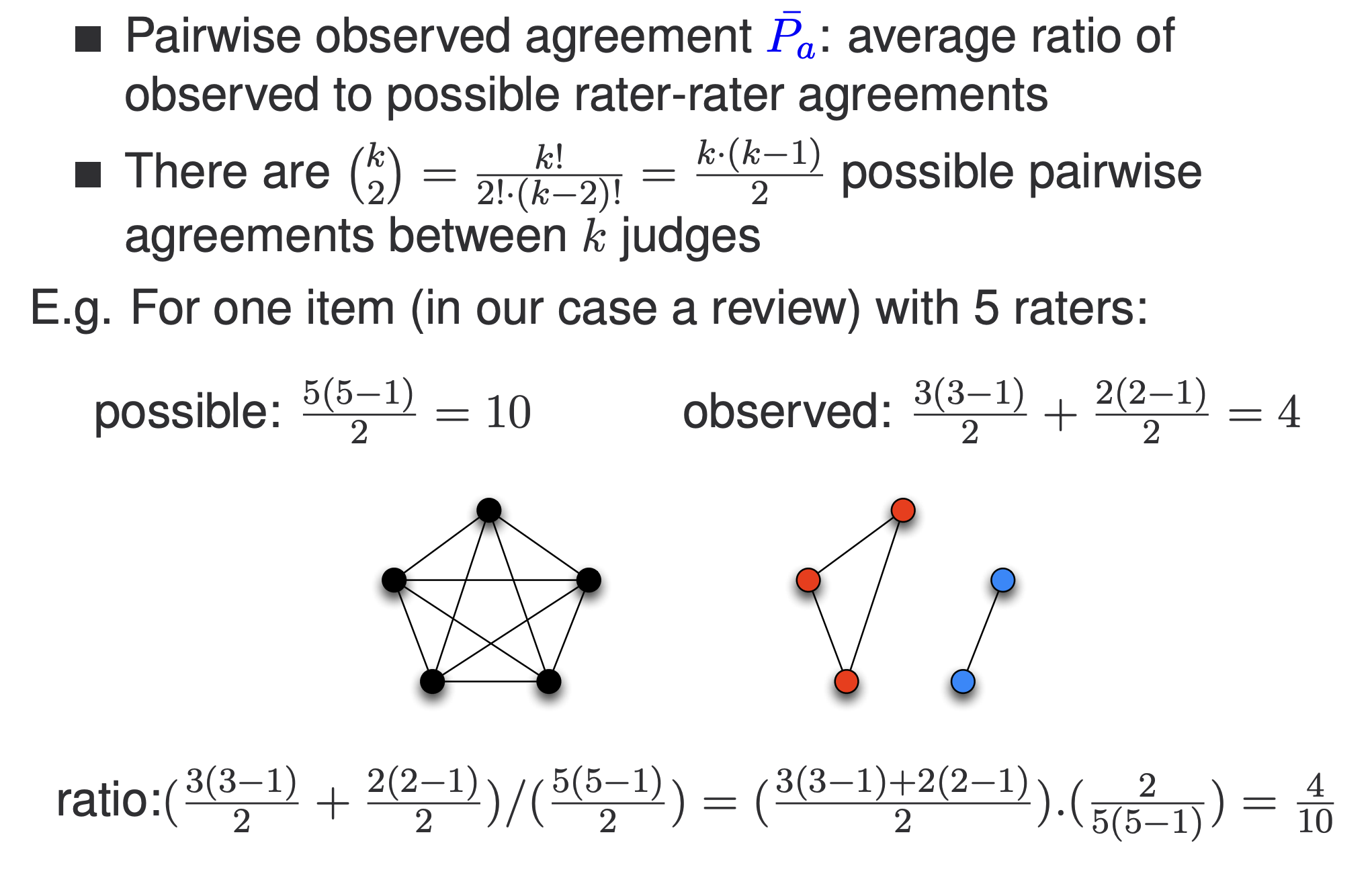
$S_i$: ratio of observed to possible pairwise agreement

$P(A)=\frac{1}{N}\sum\limits_{i-1}^NS_i$

$P(E)=\frac{1}{N}\sum\limits^n_{j=1}(\frac{C_j}{2})^2$

Interpretation of $k$ value

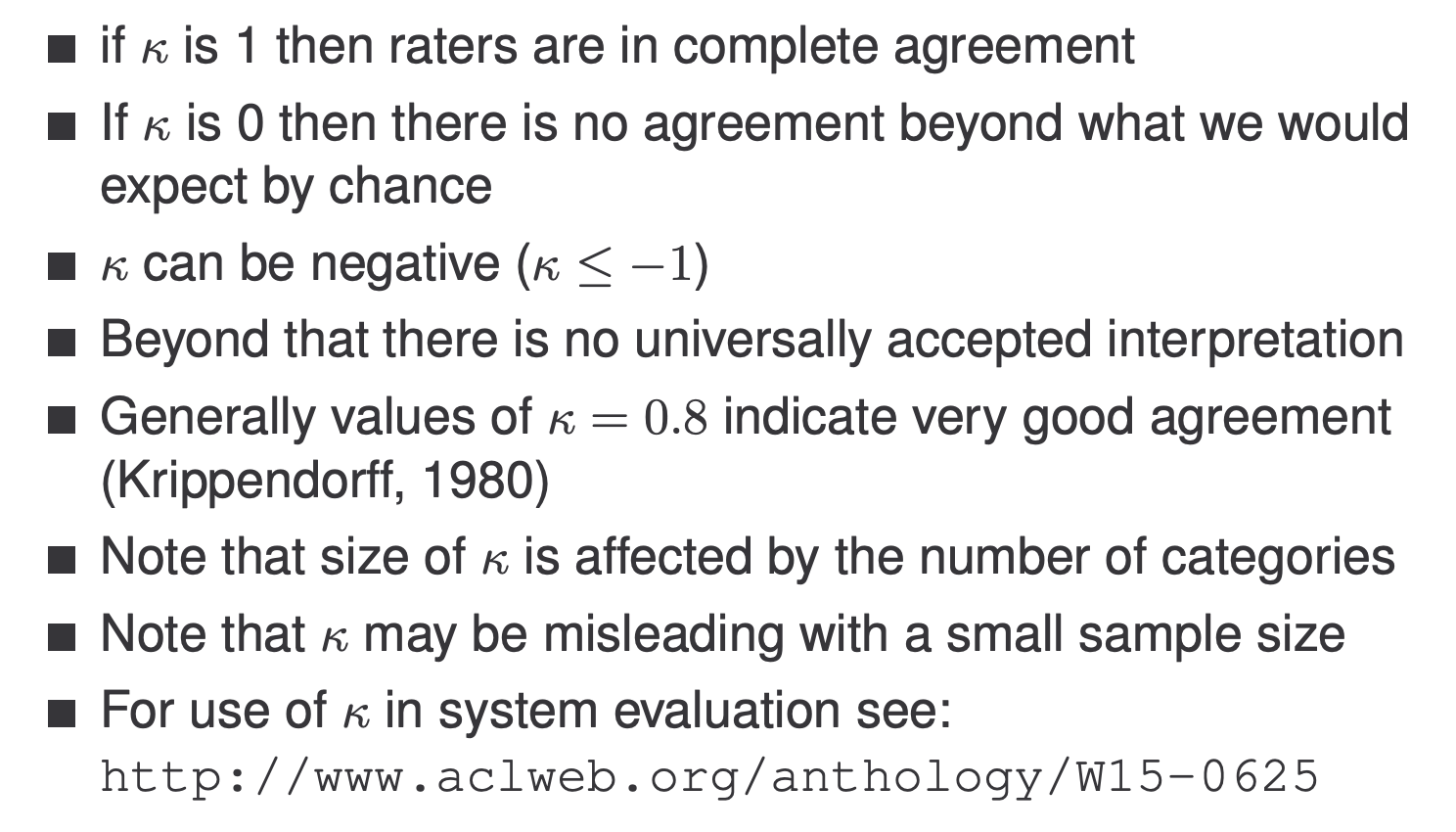
Fleiss’ Kappa is 0.65 for this set. Explain what Kappa is and outline how it is calculated. You do not need to state the full formula for Kappa.

Human annotators will not always agree on classifications. Raw agreement does not allow for the possibility that agreement might be simply a matter of chance, which is more likely in tasks with few classes. For instance, for a task with two equally balanced classes, agreement of 75% is quite low (random agreement would be 50%), while 75% agreement is quite high for a task with 10 classes. Kappa measures the agreement between annotators corrected for the possible of chance agreement. It can be calculated from a table give the classes that each annotator assigns.

Kappa of 0.65 is rather low, but should be still be usable for evaluation.

2021-p03-q09

Your colleague wants to hire two more human annotators to re-label your training data. Why might this be a good idea, how would you measure agreement in this task, and do you think this would improve your classifier in any way?

What is perceived as a threat has a large subjective component. One person’s joke is another person’s threat. It would therefore be of service if we could measure how much two people agree. To measure agreement, we can use kappa. Kappa reports only agreement above the chance level. In general tasks of this kind, majority opinion is often used. Here, if we want a sensitive classifier that picks up even hidden threats, it might be better to count something as a threat if even just one annotator decided so. This is likely to improve the classifier’s REAL recall (make it more sensitive to cyberbullying), even if the measured numbers on test would go down slightly, because cyberbulling now appears to be more frequent compared to the one-annotator situation.

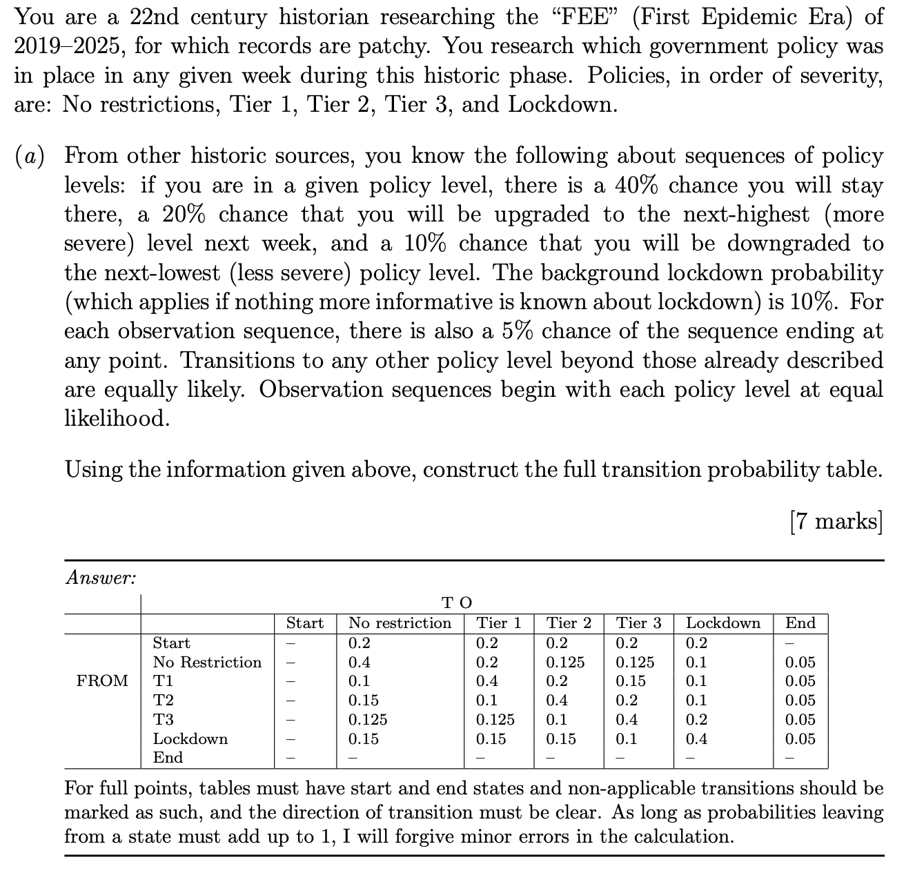
Lecture 8 (Hidden Markov Models)

Weather prediction

• Two types of weather: rainy and cloudy
• The weather doesn’t change within the day
• Can we guess what the weather will be like tomorrow?
• We can use a history of weather observations:

$$
P(w_t=Rainy|w_{t-1}=Rainy,w_{t-2}=Cloudy,w_{t-3}=Cloudy,w_{t-4}=Rainy)
$$

Properties

1. Markov Assumption(Limited Horizon): Transition only depends on current state

$$
P(X_t|X_{t-1},X_{t-2},X_{t-3},X_{t-4}…,X_{1}) \approx P(X_t|X_{t-1})
$$

The joint probability of a sequence of observations/events can then be approximated as:
$$
P(X_1,X_2,…,X_t) \approx \prod^{n}{t=1}P(X_t|X{t-1})
$$

2. Output independance

Probability of an output observation depends only on the current state and not on any other states or any other observations:
$$
P(O_t|X_1,…X_t,…,X_T,O_1,…O_t,…,O_T)\approx P(O_t|X_t)
$$

Markov Chains

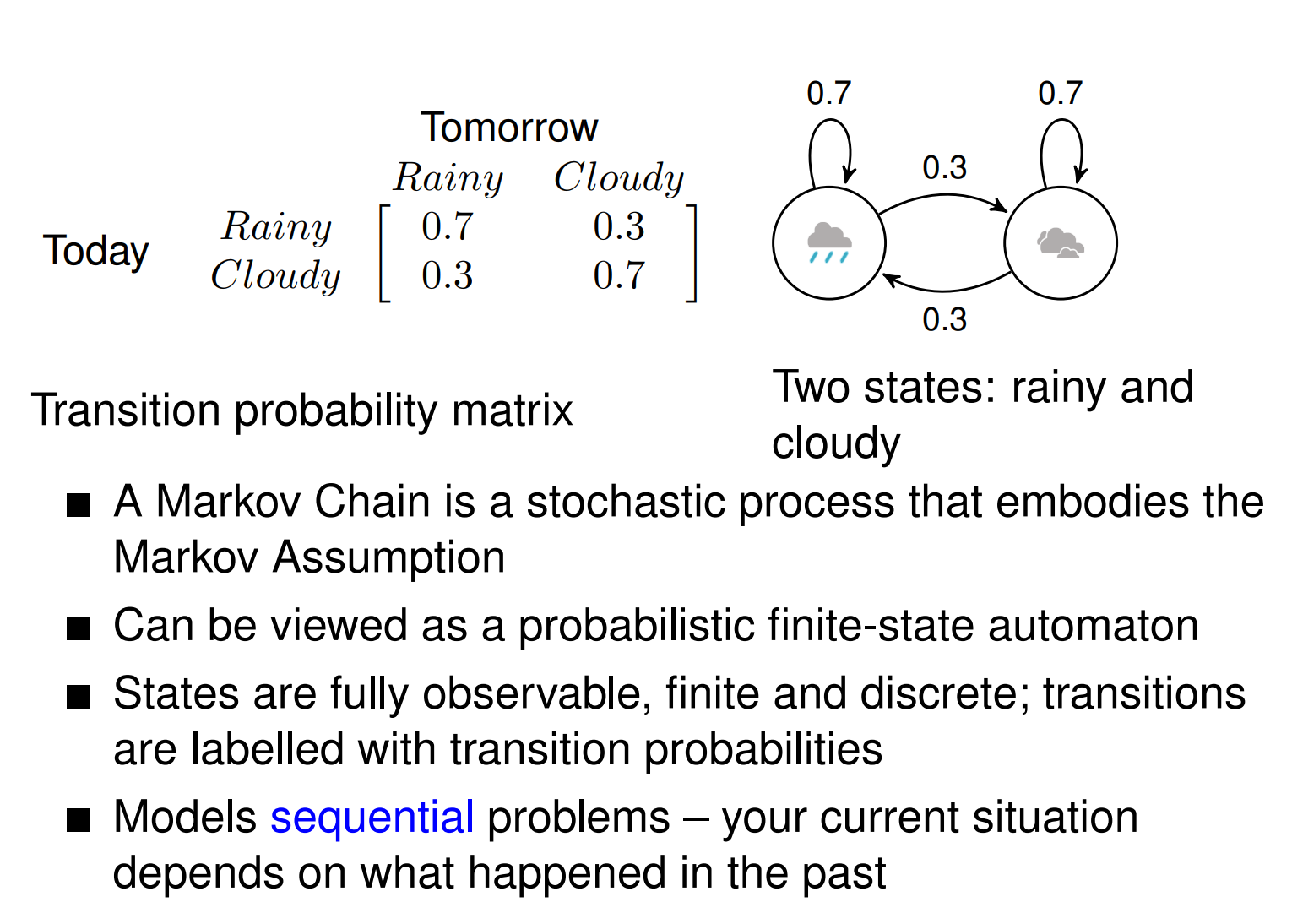
• Useful for modelling the probability of a sequence of events that can be unambiguously observed.

  • Valid phone sequences in speech recognition
  • Sequences of speech acts in dialog systems (answering, ordering, opposing)
  • Predictive texting

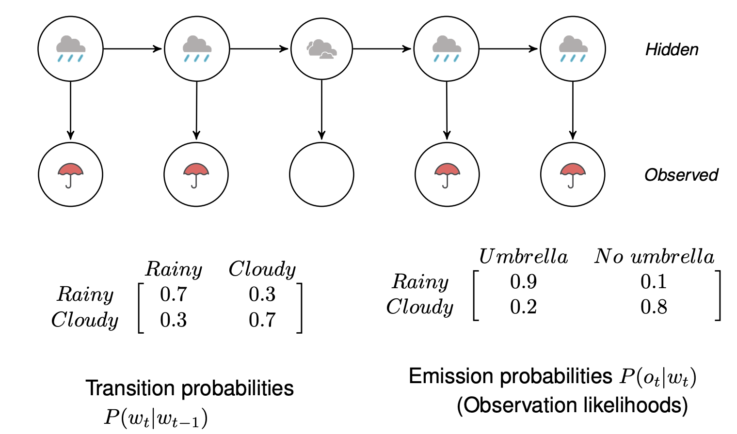
• Underlying Markov Chain over hidden states

• We only have access to the observations at each time step.

• There is no 1:1 mapping between observations and hidden states.

• A number of hidden states can be associated with a particular observation, but the association of states and observations is governed by probabilities.

• We now have to infer the sequence of hidden states that corresponds to the sequence of observations.

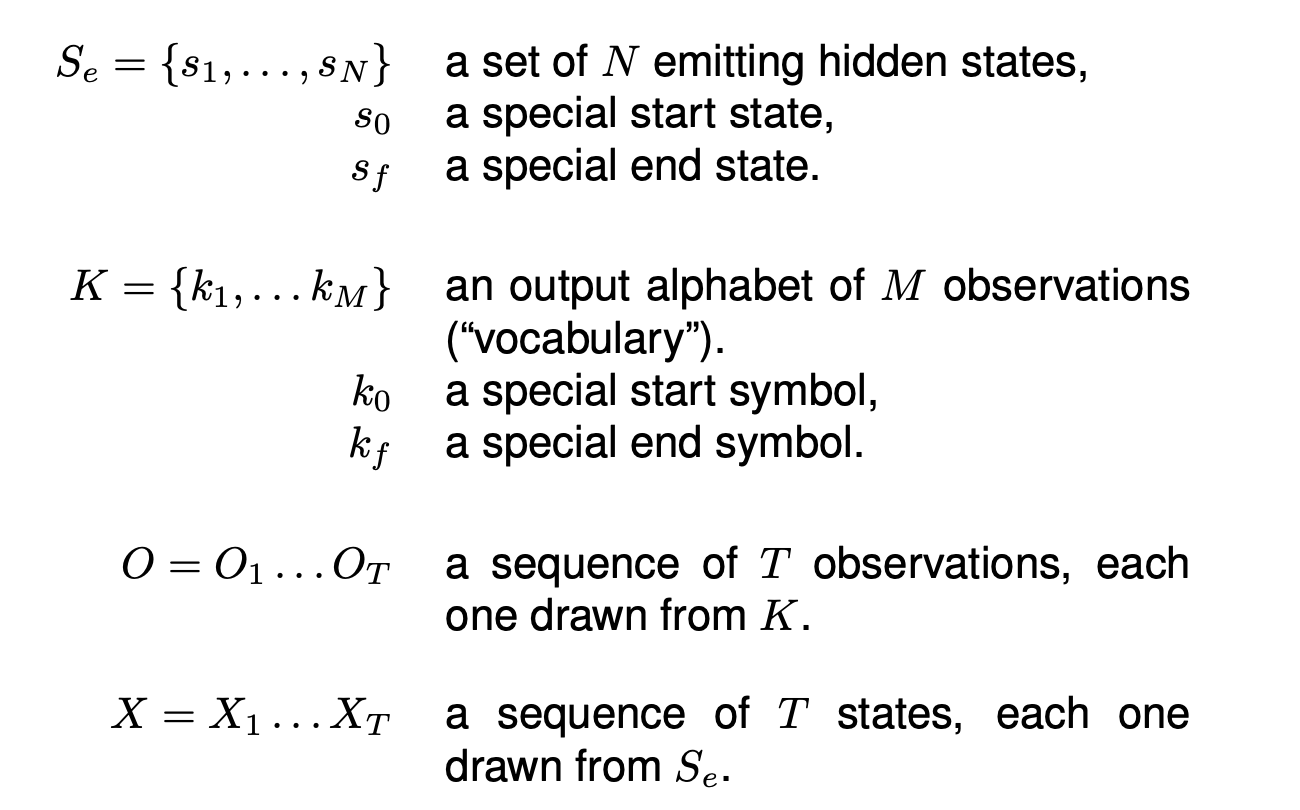
Start and End states

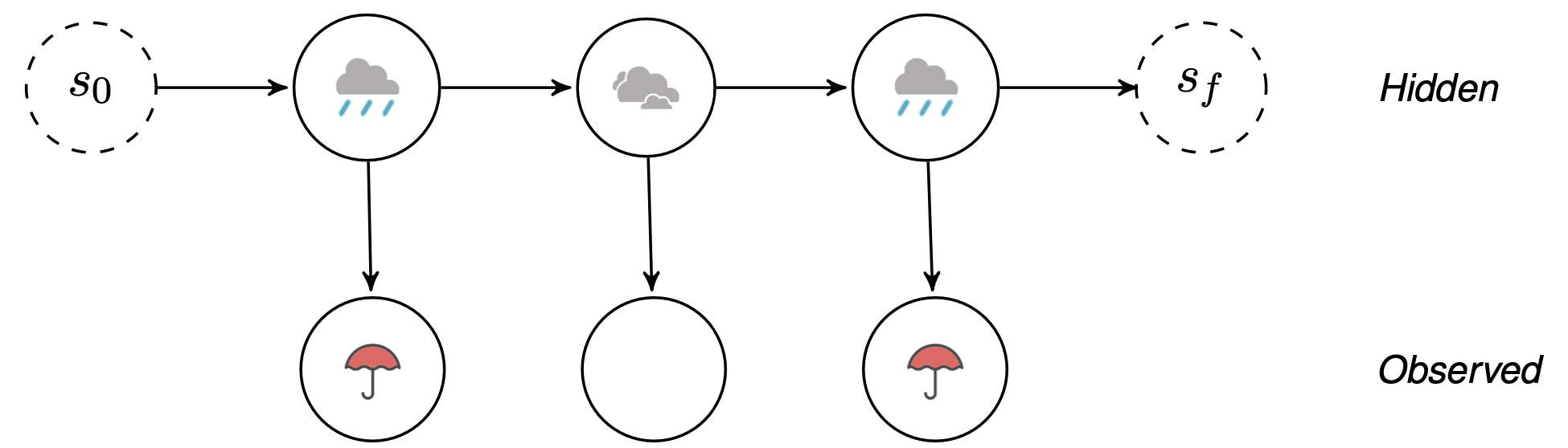
• Could use initial probability distribution over hidden states.
• Instead, for simplicity, we will also model this probability as a transition, and we will explicitly add a special start state.
• Similarly, we will add a special end state to explicitly model the end of the sequence.
• Special start and end states not associated with “real“ observations.

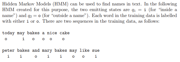
2020-p03-q08

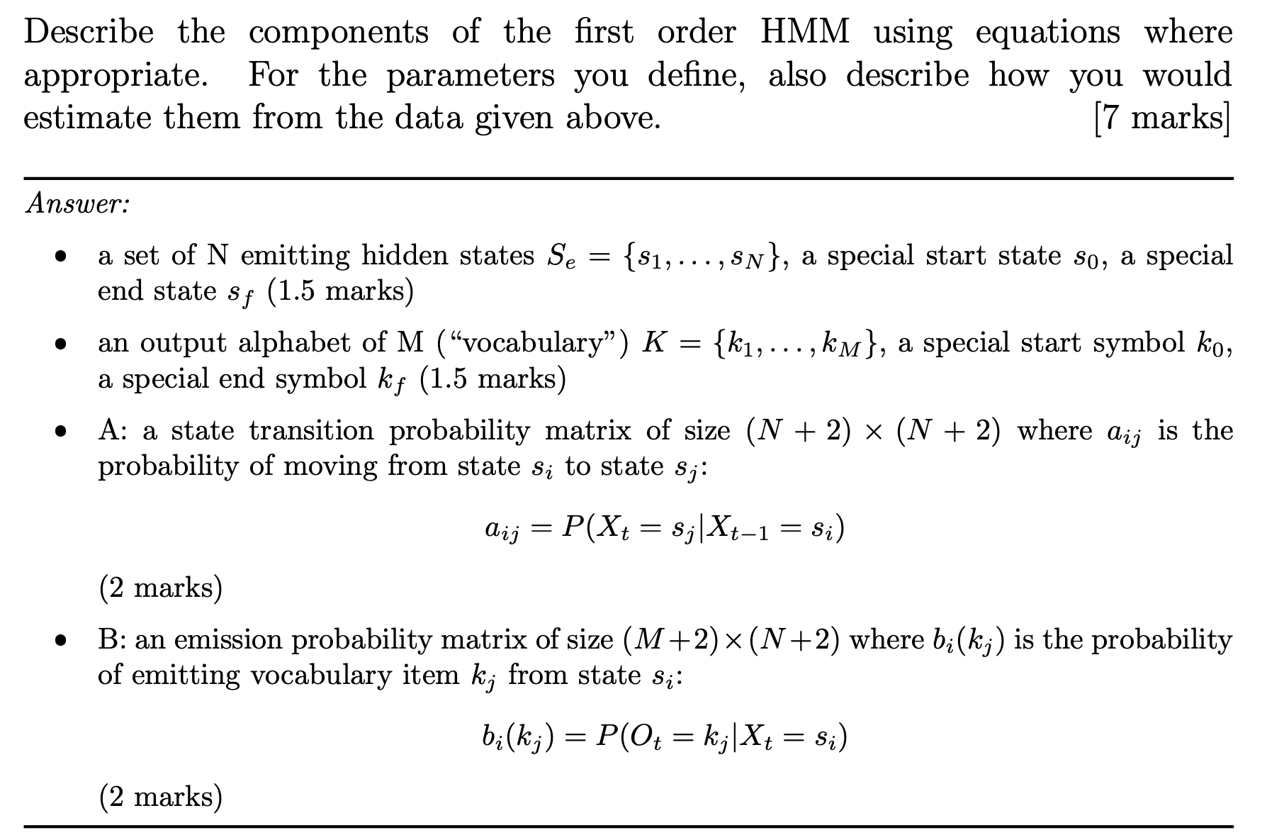
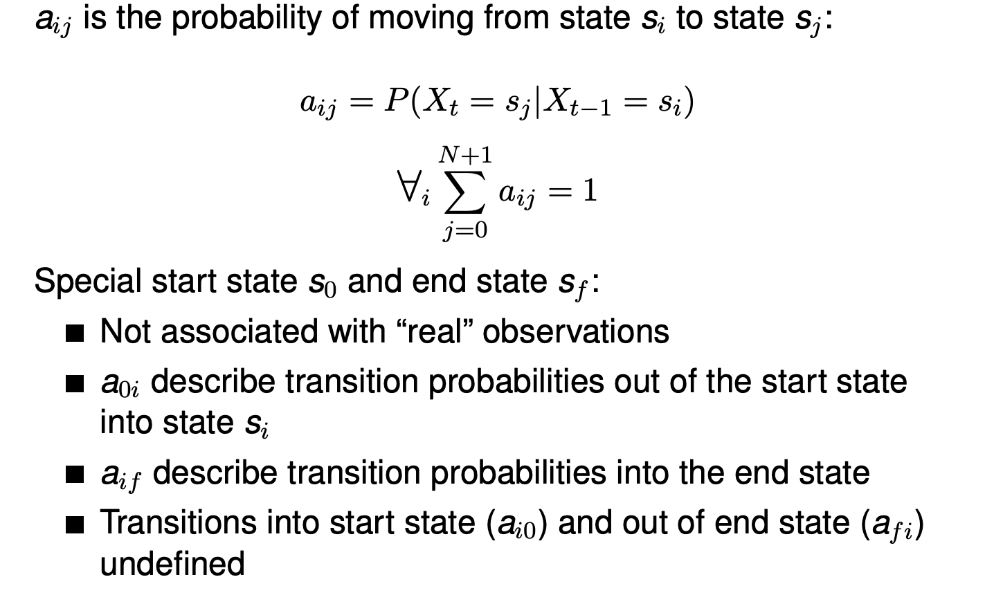
State transition probability

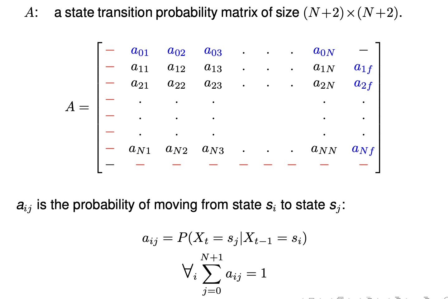
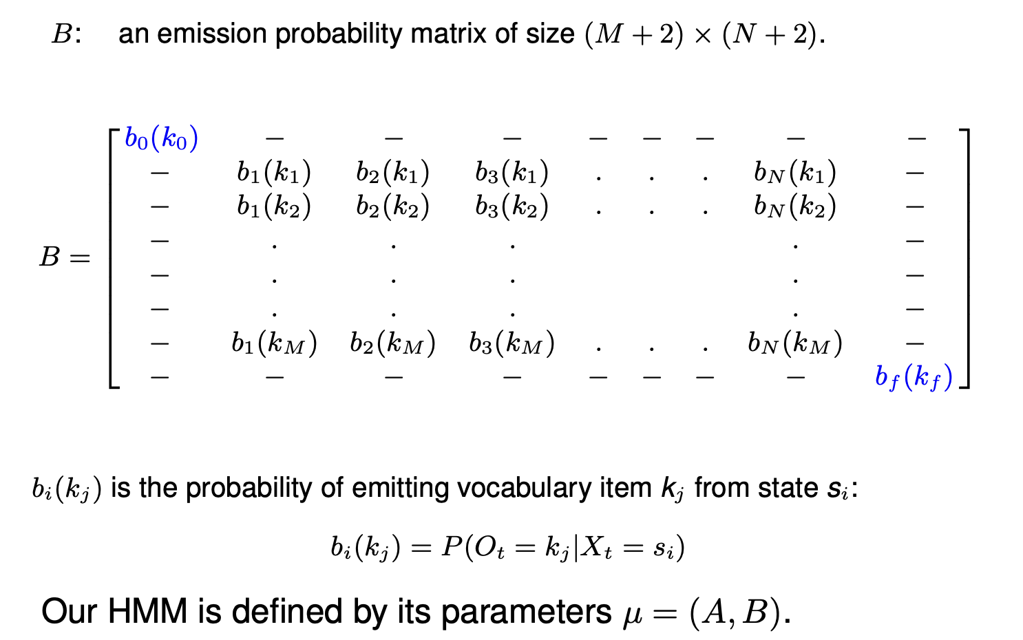
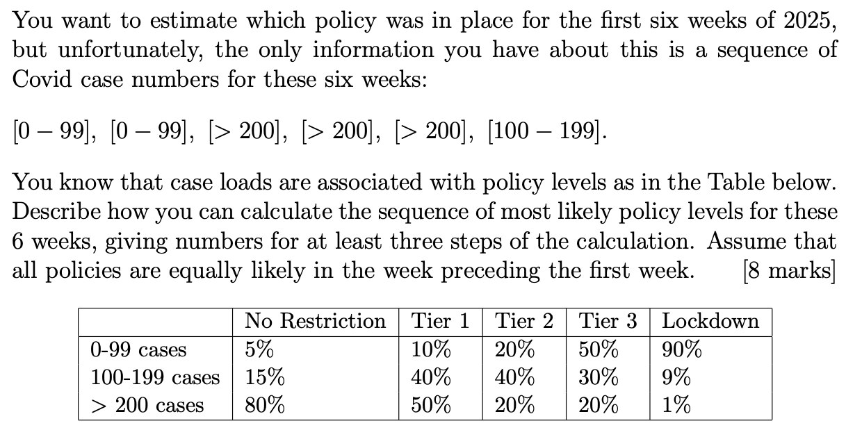
Emission probabilities

2017-p02-q09

A comparable situation can arise when estimated emission probability is 0 and thus probability assigned to a series of observation and their interpretation being 0 even when substantial amount of training data. Describe why this is a problem and indicate a solution to it

1. Heap’s Law means that test data is likely to contain words unseen in the training data, no matter how much training data we have
2. There will always be new names, and words we have seen previously will be used as names (this doesn’t follow from Heap’s law, but is a reasonable assumption). Any such case will be assigned probability 0 if we simply assign probability based on counts in the training data
3. This is also true of other phenomena: sparse data is a general problem in machine learning
4. The solution is to smooth: adjust the MLE based on the counts via an unseen probability mass and hence avoid probabilities of 0
5. The simplest technique is add-one / Laplace smoothing, which means that 1 is added to all counts (it is helpful to give the formulae in the answer).

relevant comments

• It is unlikely we will need to smooth the transition probabilities for this application
• the use of logs means we need to do something about 0 probabilities in calculation
• there are some phenomena where we may have genuine 0 probabilities, but it may be difficult to establish this
• for this application there are useful possible heuristics - e.g., capitalization

Parameter Estimation

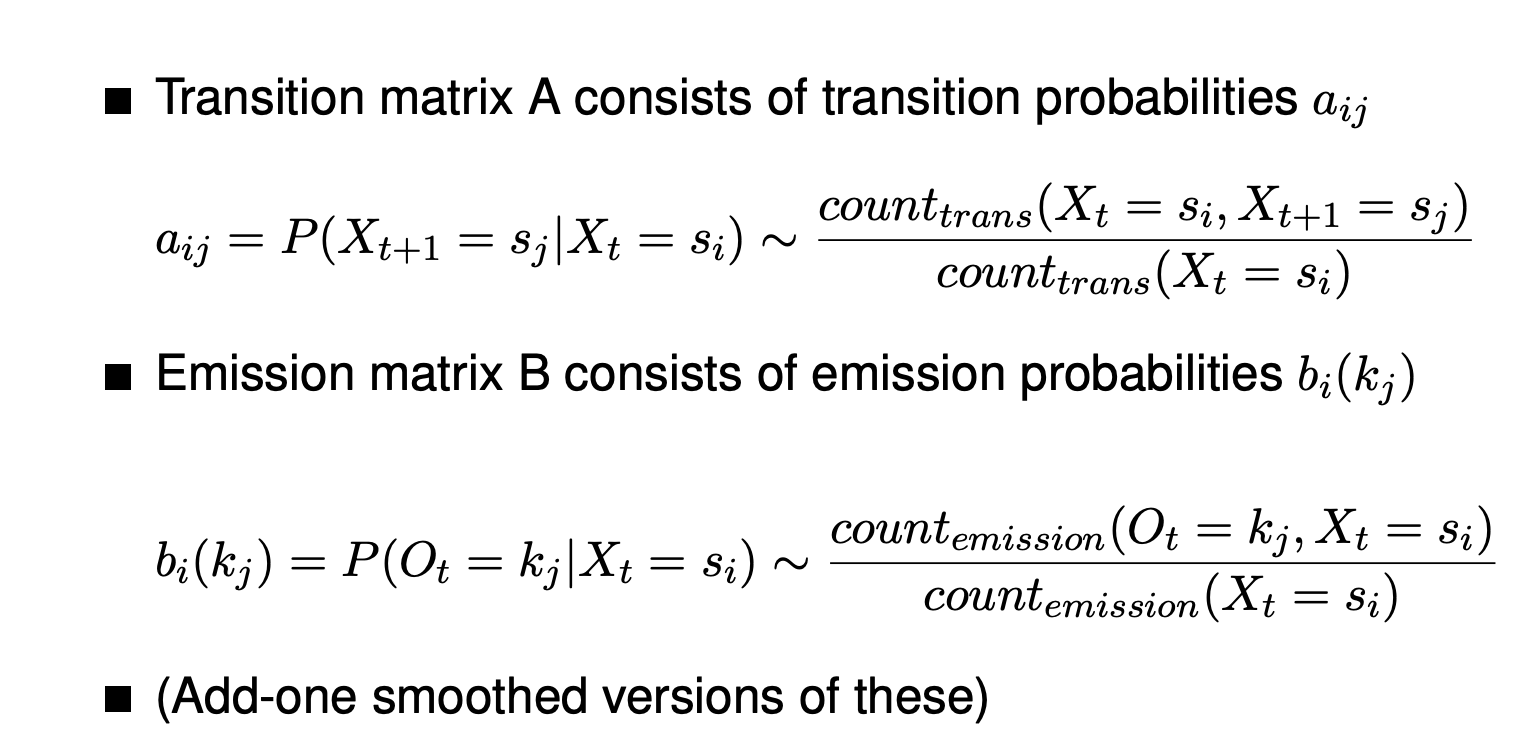
Add-one smoothed version of these

$$
a_{ij}=P(X_{t+1}=s_j|X_t=s_i)\sim \frac{count_{trans}(X_t=s_i,X_{t+1}=s_j)+1}{count_{trans}(X_t=s_i)+N}\
\text{N is the number of distinct hidden emission states}
\
b_i(k_j)=P(O_t=k_j|X_t=s_i)\sim \frac{count_{emission}(O_t=k_j,X_t=s_1)+1}{count_{emission}(X_t=S_i)+N} \
\text{N is the number of distinct obervations possible}
$$

2018-p03-q08

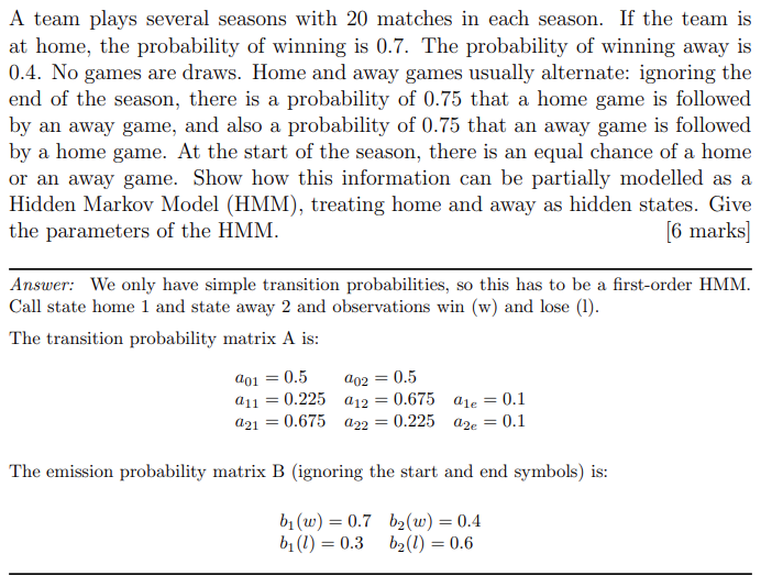
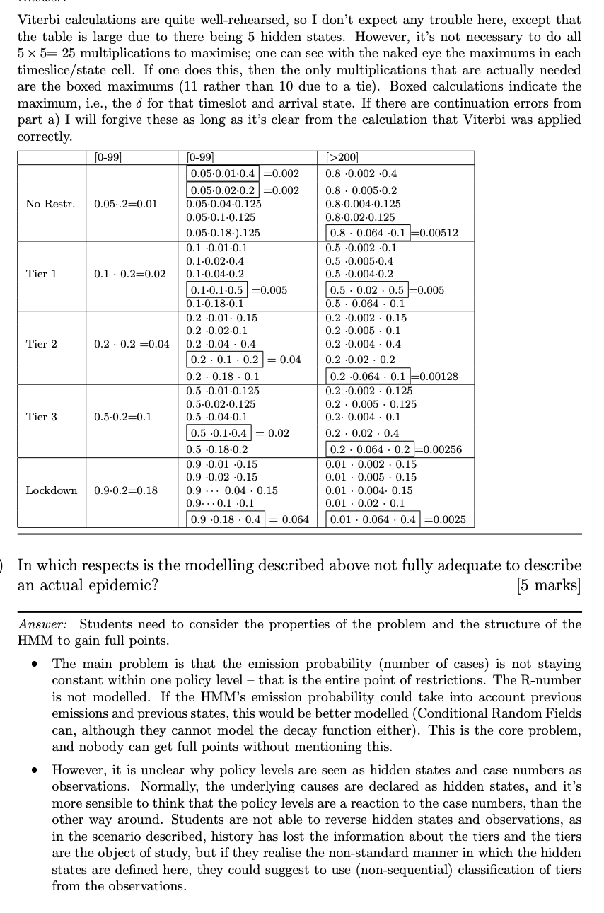
What aspect of the scenario described is not correctly covered by the HMM?

The HMM cannot model the fixed length of the season

You are given a complete record of individual games, including a record of the opponents. The win/loss ratio varies depending on the opponent. Explain how you could use such information to derive the parameters of a more complex HMM (treating home and away as hidden states, as before).

In a more complex setting where observations correspond to different events, such as winning or losing against different opponents, we need to consider these events separately.

Transition probabilities for states (for instance, from ‘home’ to ‘away’) are calculated as follows:

$$ P(\text{home} \rightarrow \text{away}) = \frac{\text{count(home} \rightarrow \text{away})}{\text{count(all transitions from home)}}$$

Emission probabilities, for example, the probability of winning at home against opponent 1, are calculated by dividing the total number of home wins against opponent 1 by the total number of home games:

$$P(\text{win against opponent 1}|\text{home}) = \frac{\text{count(home wins against opponent 1)}}{\text{count(all home games)}}$$

However, with a small number of opponents and a long sequence of games, there might be cases where a particular observation (like winning or losing against a specific opponent) was never seen in the training data.

In these cases, we would estimate its probability to be zero, which can be problematic. To avoid this, we can apply Laplace smoothing (also known as add-one smoothing), which adds a constant (usually 1) to each count:

$$ P(\text{win against opponent 1}|\text{home}) = \frac{\text{count(home wins against opponent 1)} + 1}{\text{count(all home games)} + N} $$

where N is the number of distinct observations possible. This ensures that every potential observation has a non-zero probability, even if it wasn’t seen in the training data.

It is suggested that you could use an HMM to predict the results of next season’s games, since it is known who the opponent will be and whether the match will be at home or away. How might you do this? How successful do you think this would be, compared to predicting whether a sequence of matches were home or away based on a sequence of match results?

Considering the course discussions, we can conceptualize this problem by revising our Hidden Markov Model (HMM) to have ‘win’ and ‘lose’ as hidden states. The observations would be ‘home-against-opponent-1’, ‘away-against-opponent-1‘, and so on. We can estimate the probabilities from the data, much like we did in the previous part. In this sense, it’s entirely possible to extract appropriate emission and transition probabilities from the given data.

However, there’s a potential issue with this approach. Given the scenario described, there might be relatively little information in the sequences of wins and losses. Wins and losses might tend to alternate, but this could primarily be a secondary effect of the scheduling. In such a case, there’s no point in modeling this as an HMM. We might just as well model the data as distinct events, ignoring the sequence.

To illustrate this, consider a situation where home and away matches always alternate, and the probability of winning at home is only slightly greater than the probability of winning away. In this situation, given a long sequence of matches, we can still reliably determine the home-away alternation. There are only two possibilities for the overall sequence, and the difference in winning probabilities will allow us to determine which sequence is most likely, even if the difference is very small. However, the number of sequences in terms of match results is $2^n$, where $n$ is the number of matches.

2020-p03-q08

Fundamental tasks with HMMs

Problem 1 (Labelled Learning)
Given a parallel observation and state sequence O and X, learn the HMM parameters A and B

Problem 2 (Unlabelled Learning)
Given an observation sequence $O$ (and only the set of emitting states $S_e$), learn the HMM parameters A and B

Problem 3 (Likelihood)
Given an HMM μ = (A, B) and an observation sequence O, determine the likelihood $P(O|\mu)$

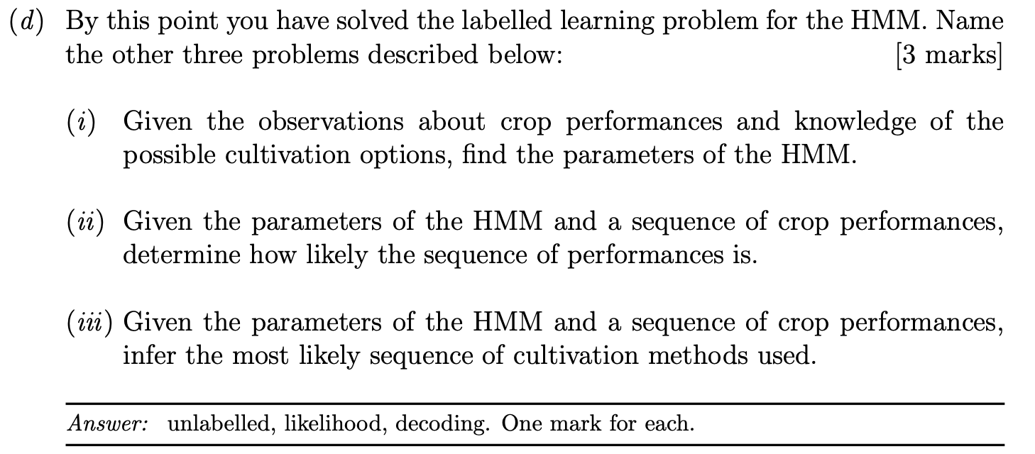
Problem 4 (Decoding)
Given an observation sequence O and an HMM μ = (A, B), discover the best hidden state sequence X → Task 8

Lecture 9: Viberti Algorithm for HMM decoding

Decoding

Verbiti

Intuition Behind

• Here’s how we can save ourselves a lot of time.
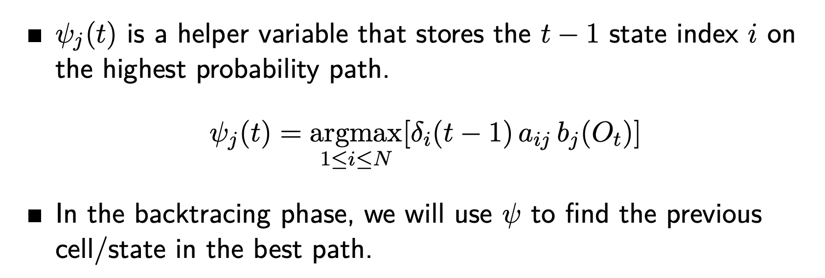
• Because of the Limited Horizon of the HMM, we don’t need to keep a complete record of how we arrived at a certain state.
• For the first-order HMM, we only need to record one previous step.
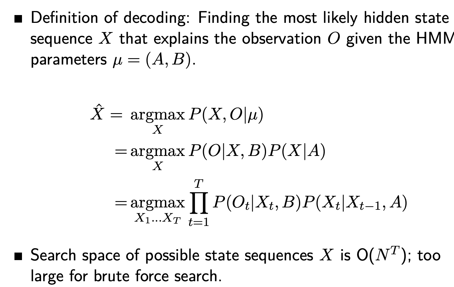
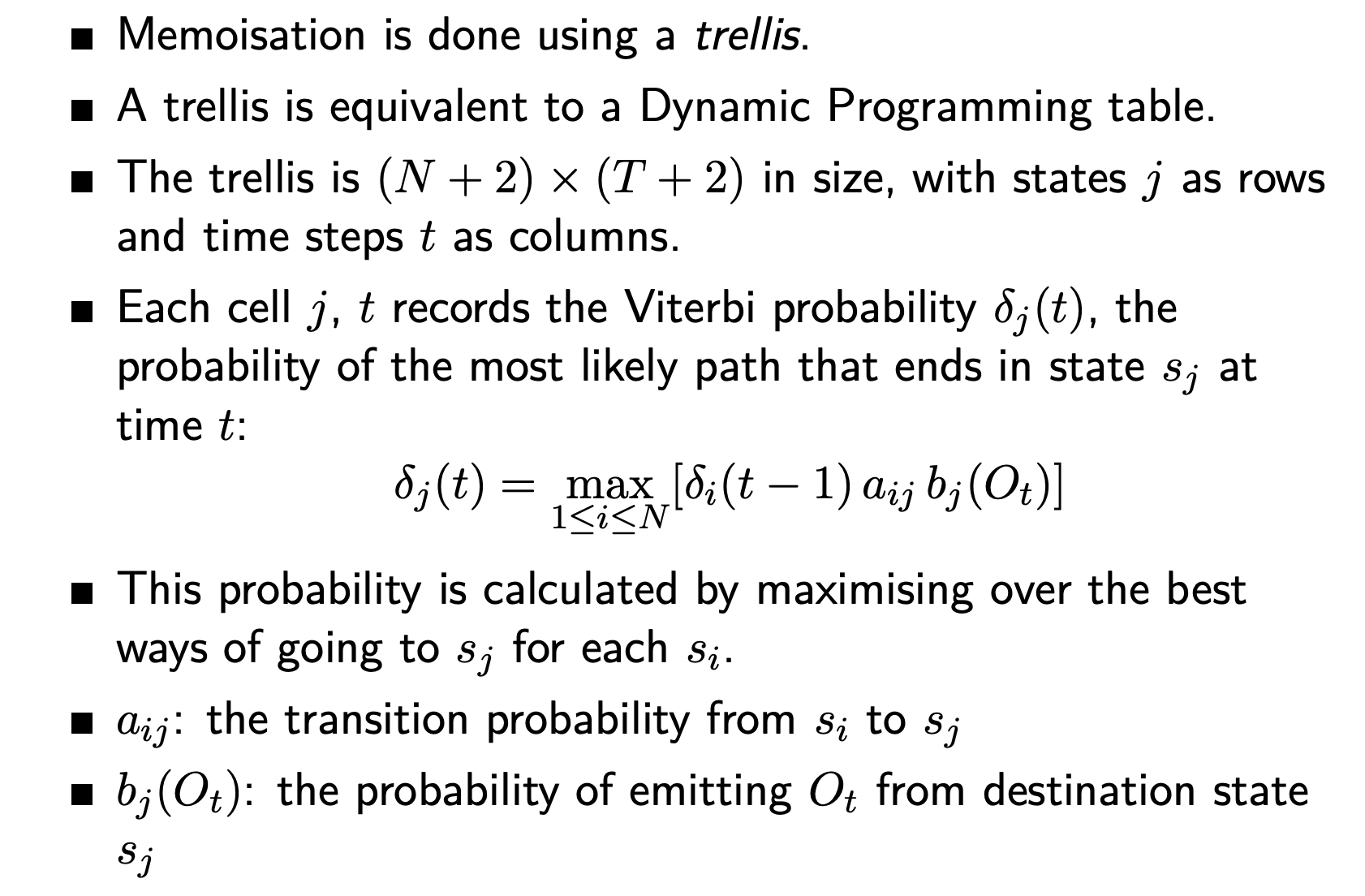
• Just do the calculation of the probability of reaching each state once for each time step (variable $\delta$).
• Then memoize this probability in a Dynamic Programming table.
• This reduces our effort to $O(N^2T)$.
• This is for the first-order HMM, which only has a memory of one previous state.

2021-p03-q08

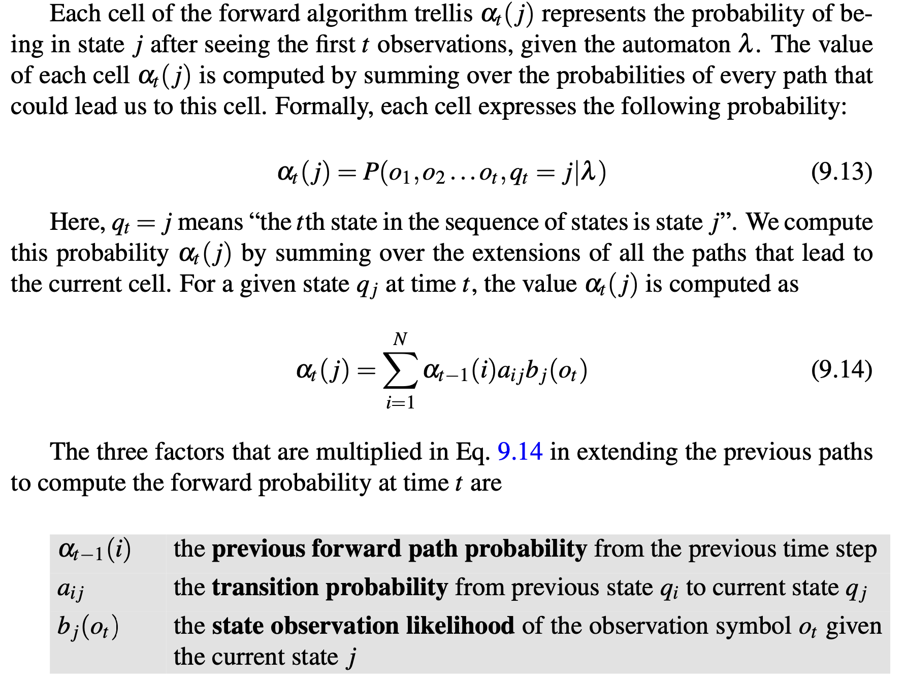
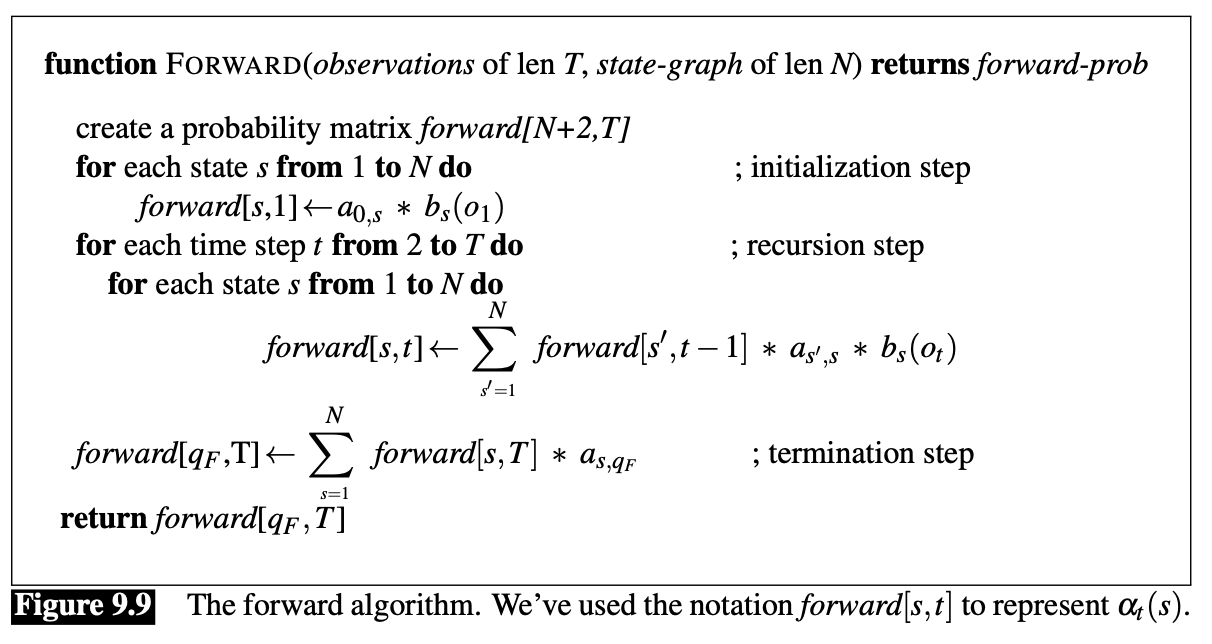
Forward Algorithm

$O(N^2T)$ time complexity

Precision and recall

Lecture 12 (Social Networks)

Definitions

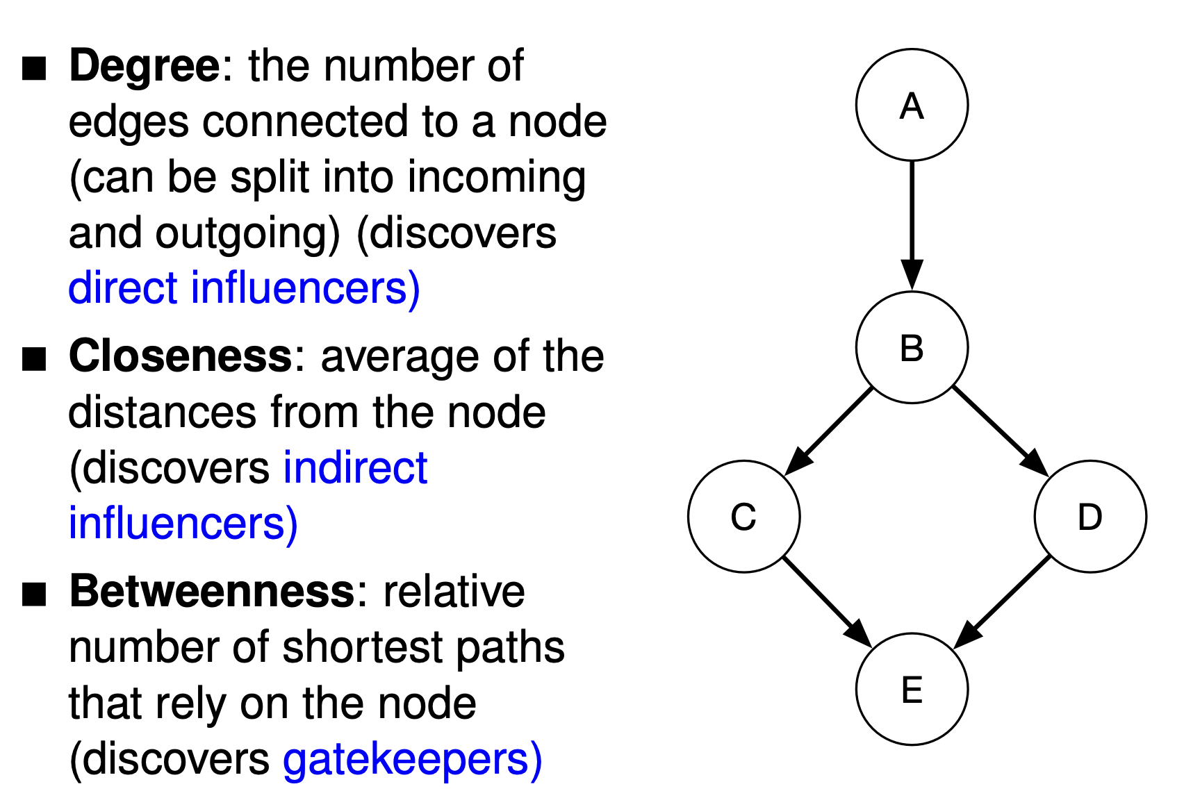
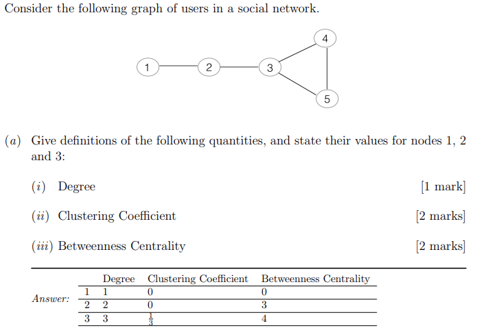
Degree: $D(v)$ = number of links of node v

Clustering coefficient = number of edges between pairs of neighbours of node v, divided by number of pairs of neighbours of node v
$$
\frac{\text{number of edges between pairs of neighbours of node v}}{\text{number of pairs of neighbours of node v}}
$$
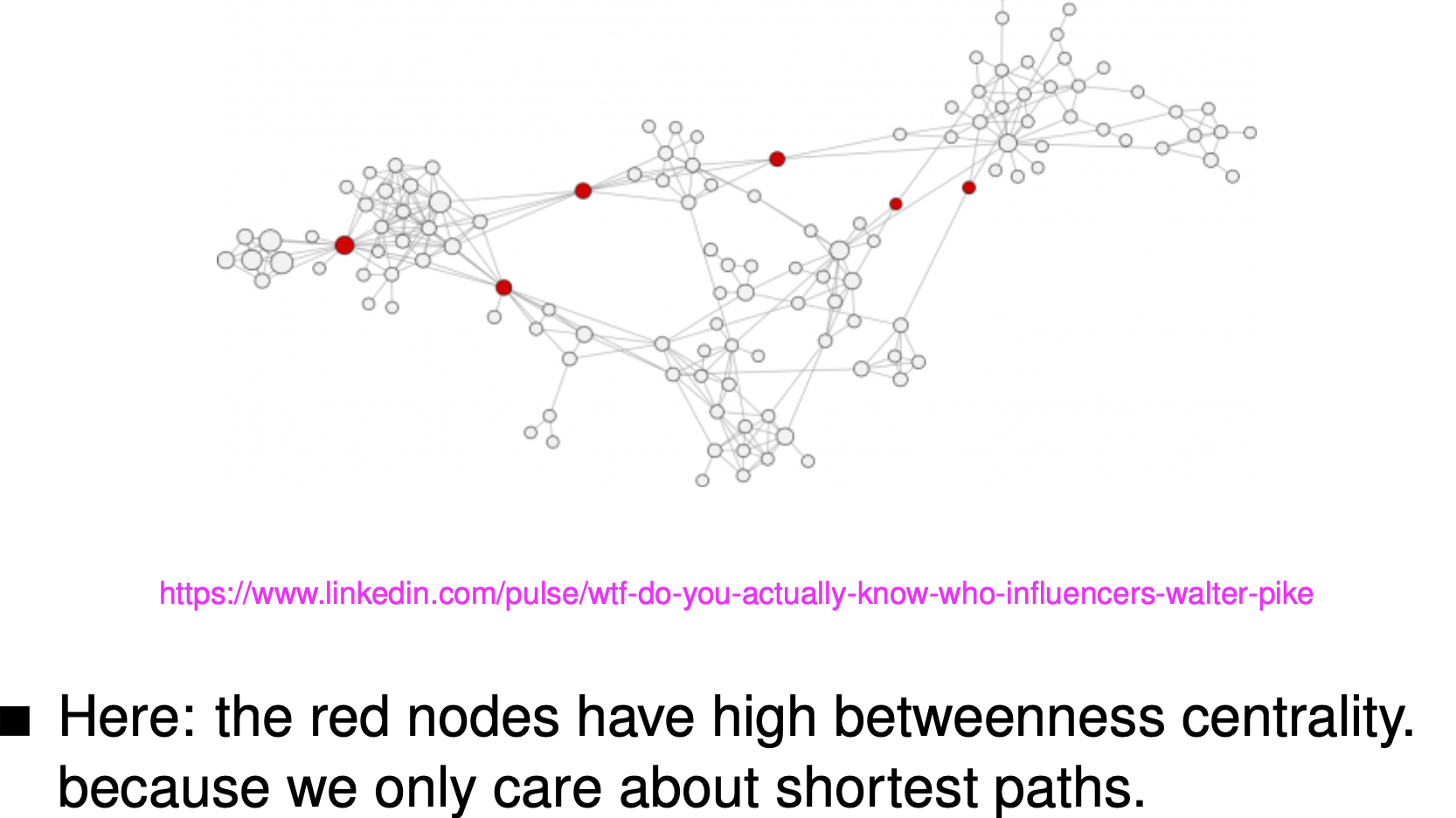
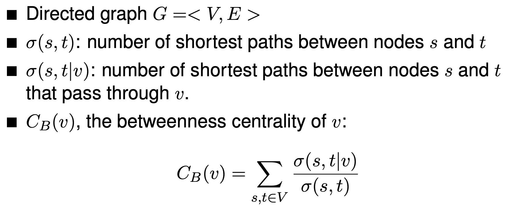
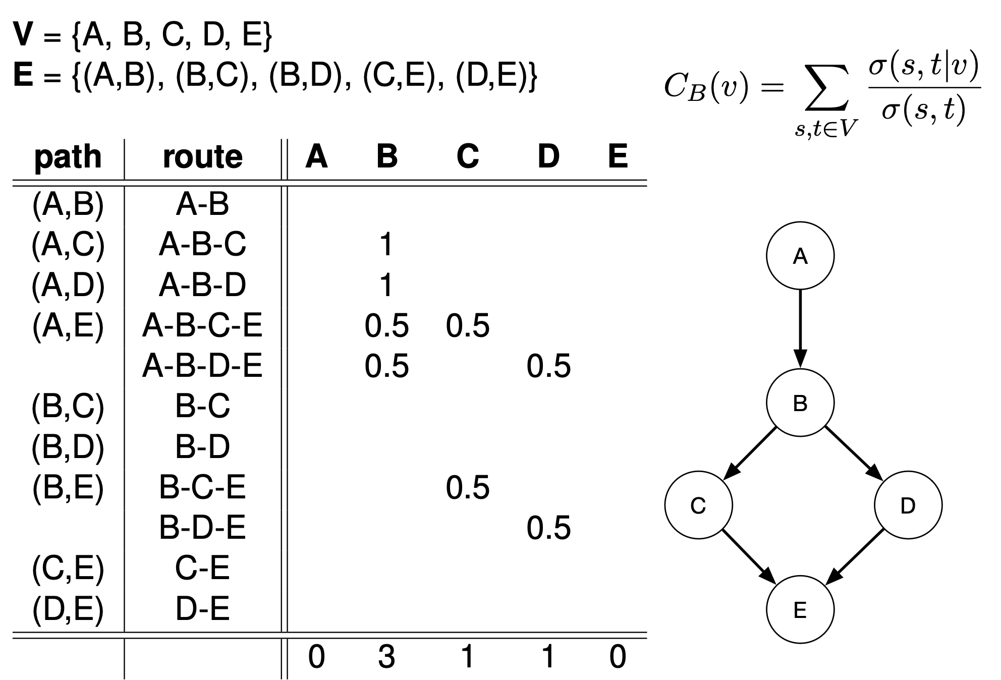
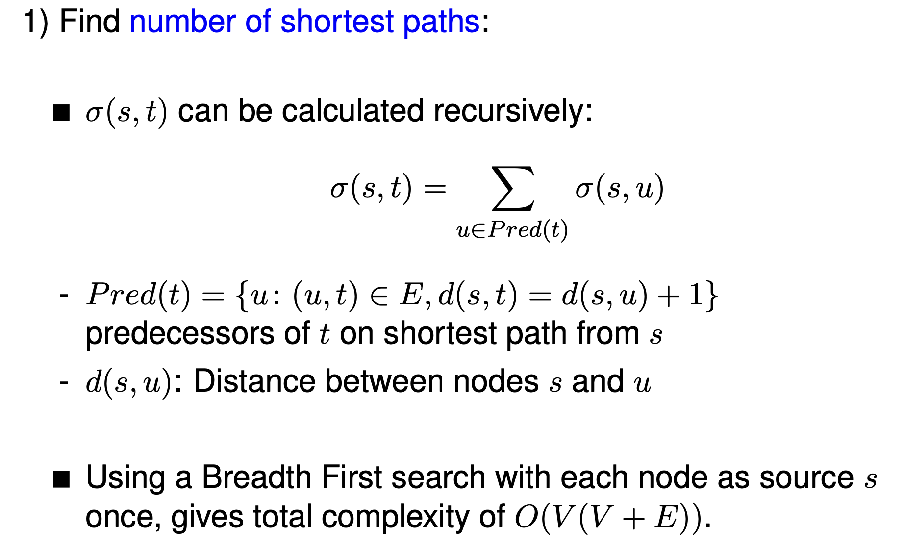
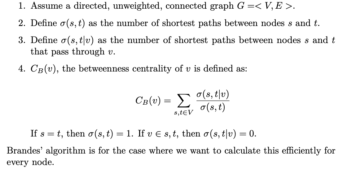
Betweenness Centrality $C(v)=\sum_{s\ne t \ne v}\frac{\sigma_{st}(v)}{\sigma_{st}}$ (proportion of shortest paths in graph that use v to all shortest paths in the graph), with $\sigma_{st}$ being the number of shortest path between two nodes $s,t$ and $\sigma_{st}(v)$ being the number of shortest paths between nodes $s$ and $t$ that contains $v$.

Let V be the set of nodes in the graph, let $\sigma(a,b)$ be the number of shortest paths from a to b, let $\sigma(a,b|v)$ be the number of shortest path from a to b that goes through v. The betweenness centrality of a node v is:
$$
\sum_{a\ne b \ne v}\frac{\sigma(a,b|v)}{\sigma(a,b)}
$$
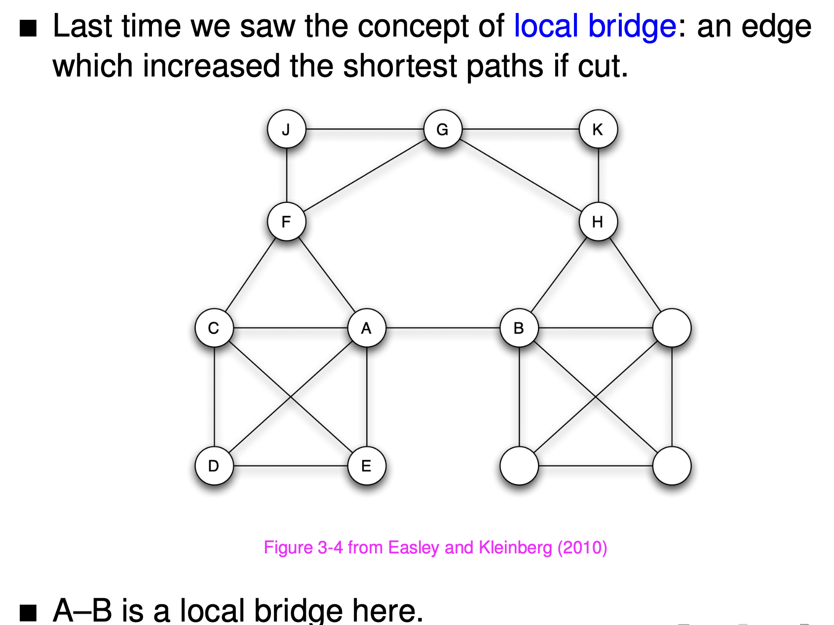
Diameter is the longest of the shortest paths between pairs of node.

Bridge: A bridge is an edge that connects two nodes that would otherwise be in disconnected components of the graph

Local bridge: A local bridge is an edge joining two nodes that have no other neighbours in common. Call the nodes connecting to the central node the gatekeeper nodes, the local bridges are the edges connecting these nodes to the central node.

Shortest path: In the case of an unweighted graph, it is the paththat connects two nodes with the fewest edges

Strongly connected: Directed graphs are called strongly connected if there exists a path from every node to every other node.

Closeness: average of the distances from the node

Which property of nodes in a network do clustering coefficient and betweenness centrality attempt to model? Give examples from naturally occurring networks.

Clustering coefficient models the degree to which a node is a “hub” between unconnected neighbours, or centre of a tightly-knit network. In social networks, when your friends become friends of your friends, your clustering coefficient goes up.

Betweenness centrality of a node models the bridge functionality of the node – the degree to which the node controls access relatively tighter-knit areas of the network. In a social network, nodes with high betweenness are the connectors between social circles who are not part of the social circles, but are the only ones that provide access to the circle.

Clustering

Social networks

Examples

Facebook-style networks:

• Nodes: people; Links: “friend”, messages

Twitter-style networks:

• Nodes: Entities/people Links: “follows”, “retweets” Also: research citations

Reasons to analyse social network

• Academic investigation of human behaviour (sociology, economics etc)

• Disease transmission in epidemics.

• Modelling information flow: e.g., who sees a picture, reads a piece of news (or fake news).

• Identifying links between subcommunities, well-connected individuals:

  • novelty

  • targeted advertising . . .

• Lots of applications in conjunction with other approaches: e.g., sentiment analysis of tweets plus network analysis.

Modelling

Networks are modelled as graphs: undirected and unweighted here.

• distance is the length of shortest path between two nodes.

• diameter of a graph: maximum distance between any pair of nodes

• degree of a node: the number of neiboughers the node has in the graph

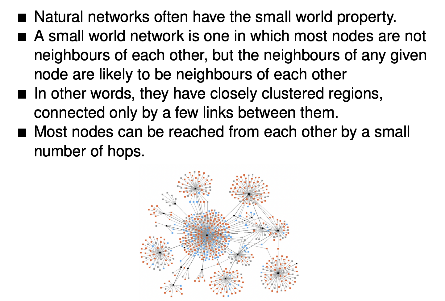
Small world phenomenon

2020-p03-q09

(Important) Concepts

• giant component: a connected component containing most of the nodes in a graph.
• weak ties: socially distant ties, infrequent interaction (acquaintances) vs. strong links: close friends and family.
• The links that keep giant components together are often only weak ties.

• bridge: an edge that connects two components which would otherwise be unconnected.
• local bridge: an edge joining two nodes that have no other neighbours in common. Cutting a local bridge increases the length of the shortest path between the nodes.
• triadic closure: if A knows B and A knows C, relatively likely B and C will (get to) know each other.
• The global clustering coefficient is a measure of the amount of triadic closure in a network.
  • It is the number of closed triads over the total number of triads (both open and closed).
• Clustering coefficient of a node A is the probability that two randomly selected neighbours of A are also neighbours of each other.

Erdős–Rényi model

The Erdős–Rényi model (1959) of random undirected graph generation is that $G_{n,p}=(V,E)$, where $n$ is the number of vertices $|V|$ and the probability of forming an edge $(u,v)∈E$ (where $u≠v$) is given by $p$. (A variant is to generate all possible graphs with the given number of vertices and edges and select between them with uniform probability, but this variant is not now used much.)

Watts-Strogatz model

The Watts-Strogatz model (1998) describes a graph $G_{n,k,p}=(V,E)$ where $n$ is the initial degree of a node (an even integer) and $p$ is a rewiring probability. It starts with a ring of nodes, with each node connected to its $k$ nearest neighbours with undirected edges (a ring lattice). Each of the starting edges $(u,v)$is visited in turn ($u<v$, starting with a circuit of the edges to the nearest neighbours, then to the next nearest and so on) and replaced with a new edge $(u,v′)$ with probability $p$. $v′$ is chosen randomly, duplicate edges are forbidden, but original edges may end up being reinstated. If p is 0, there is no rewiring, if p is 1, every edge is rewired randomly (although slightly differently from Erdős–Rényi).

Watts and Strogatz (1998) make the additional stipulation that $n≫k≫ln(n)≫1$ where $k≫ln(n)$guarantees that the graph will be connected.

Note that Easley and Kleinberg’s informal description is unlike Watts-Strogatz in not starting from a ring lattice and in not removing edges. Easley and Kleinberg discuss a variant of Watts-Strogatz (due to Kleinberg, 2000) where the random links are generated with probability proportional to the inverse square of the distance between two nodes. There are many other additional models.

Lecture 13

Centrality concepts

Node betweenness centrality

The betweenness centrality of a node V is defined in terms of the proportion of shortest paths that go through V for each pair of nodes.

---

In the network depicted above, do the betweenness centrality values you calculated correspond to your intuition about the function of nodes 1, 2, and 3? If not, which factors of the formula are responsible for the divergence?

The value for node 1 is expected. In any network, nodes at the periphery of the graph will always receive low betweenness values (0 in the special case of degree = 1, as in that case there exists no other node that can use the current node to form a shortest path). (I have given here more detail than is required.)

The values for nodes 2 and 3 are not expected, as nodes with high betweenness often have a low degree. Node 2 is on a and thus intuitively seems to have more of a bridge function than node 3, but nodes towards the centre of the entire graph also have a higher chance of aquiring a high betweenness, all other things being equal. There is a relatively high traffic in the 3-4-5 cluster, which node 2 is excluded from, and of course paths that contain the node 2 itself are excluded from the calculation. These factors result in the relatively low betweenness of node 2.

Normally, being part of a subcluster also means lower betweenness, but in the case of node 3, it is only marginally part of the cluster. Also, its more central location in the overall graph more than counteracts the disadvantage of begin part of a subcluster. The central location allows for a combinatorically growing number of paths whose end nodes lie on opposite sides of node 3

Suppose the link between 3 and 4 is removed and a link between 2 and 4 is added. How does this affect the betweenness centrality of 2 and 3, and why?

Betweenness centrality of node 2 increases to 3.5 (1–4; 1–5; 1–3; plus half of 3–4), but betweenness for node 3 drops to 1/2 + 1/2 = 1 (half of 1–5 and half of 2–5).

In other words, node 3 has now lost its overall more central position in the graph to node 2, and has become a full part of the cluster 2-3-4-5. Both changes have affected its betweenness centrality negatively.

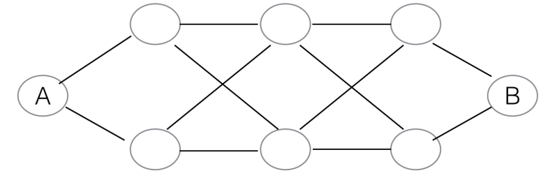
Professor Miller claims that it is possible for a particular pair of nodes in a graph to be connected by a number of shortest paths which is exponential with respect to the number of nodes in the graph. Give an example where this is the case, or prove that it cannot be the case.

Nodes A and B have $2^3$ shortest paths between them, in general $2^n$. This example can be extended infinitely. To increase $n$, add a new layer of two interleaved nodes to the graph.

---

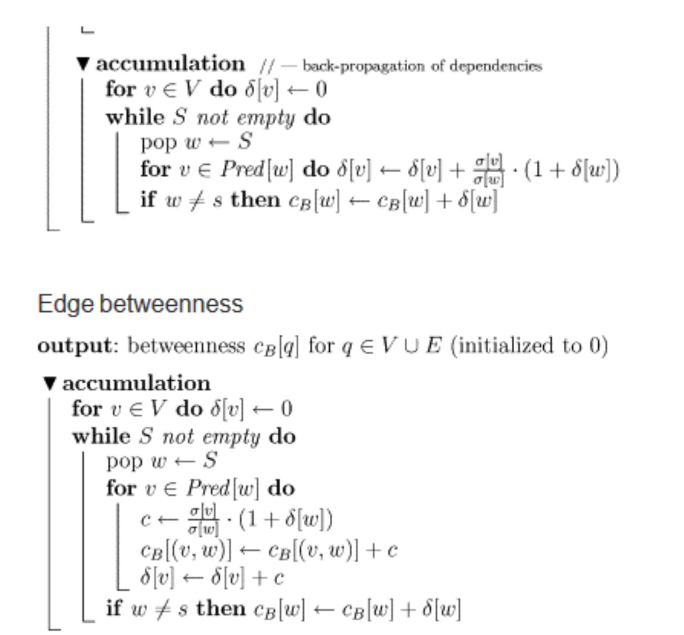
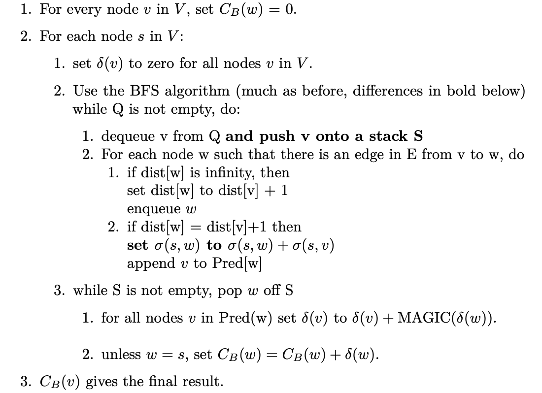
Calculating betweenness with Brandes

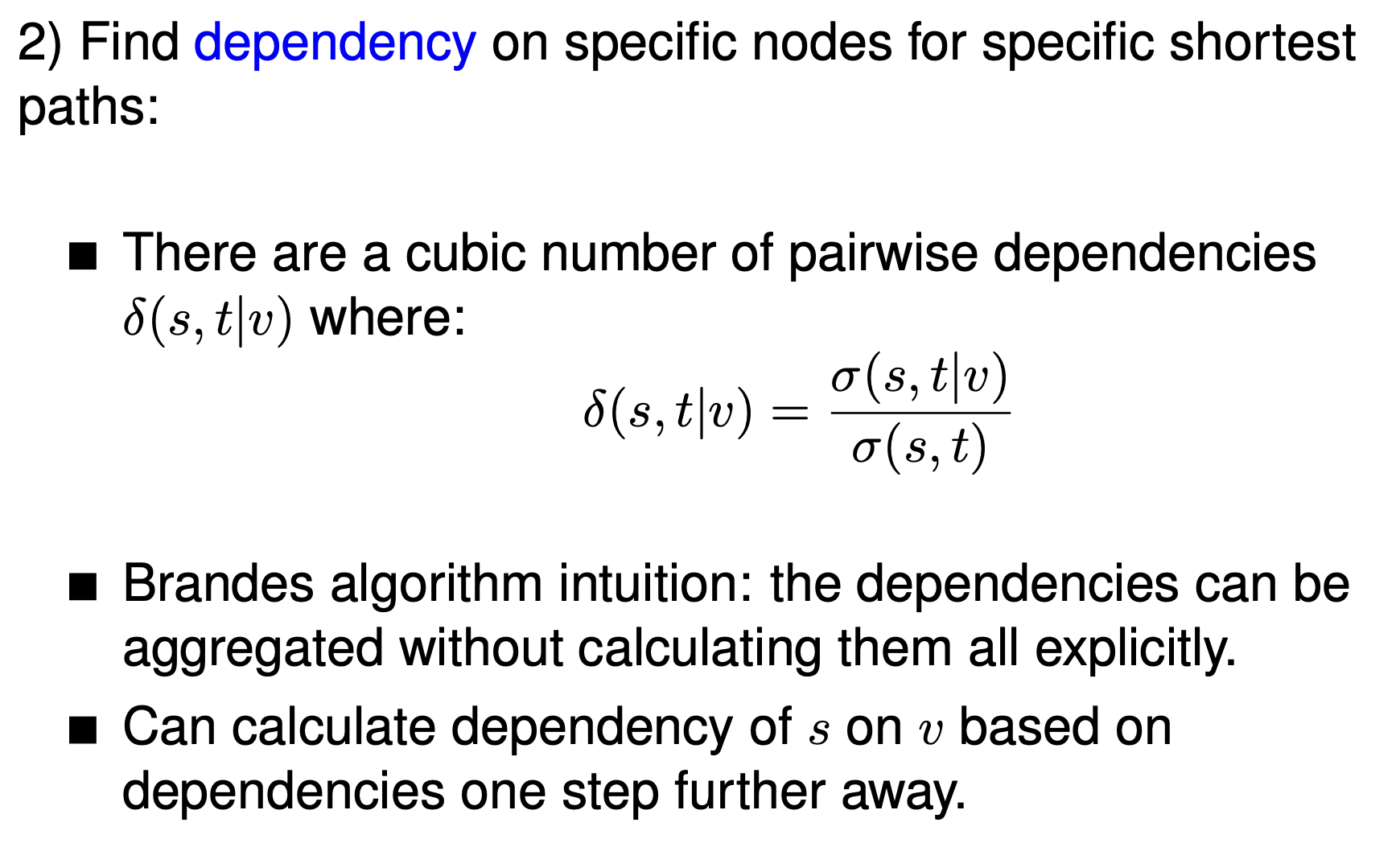
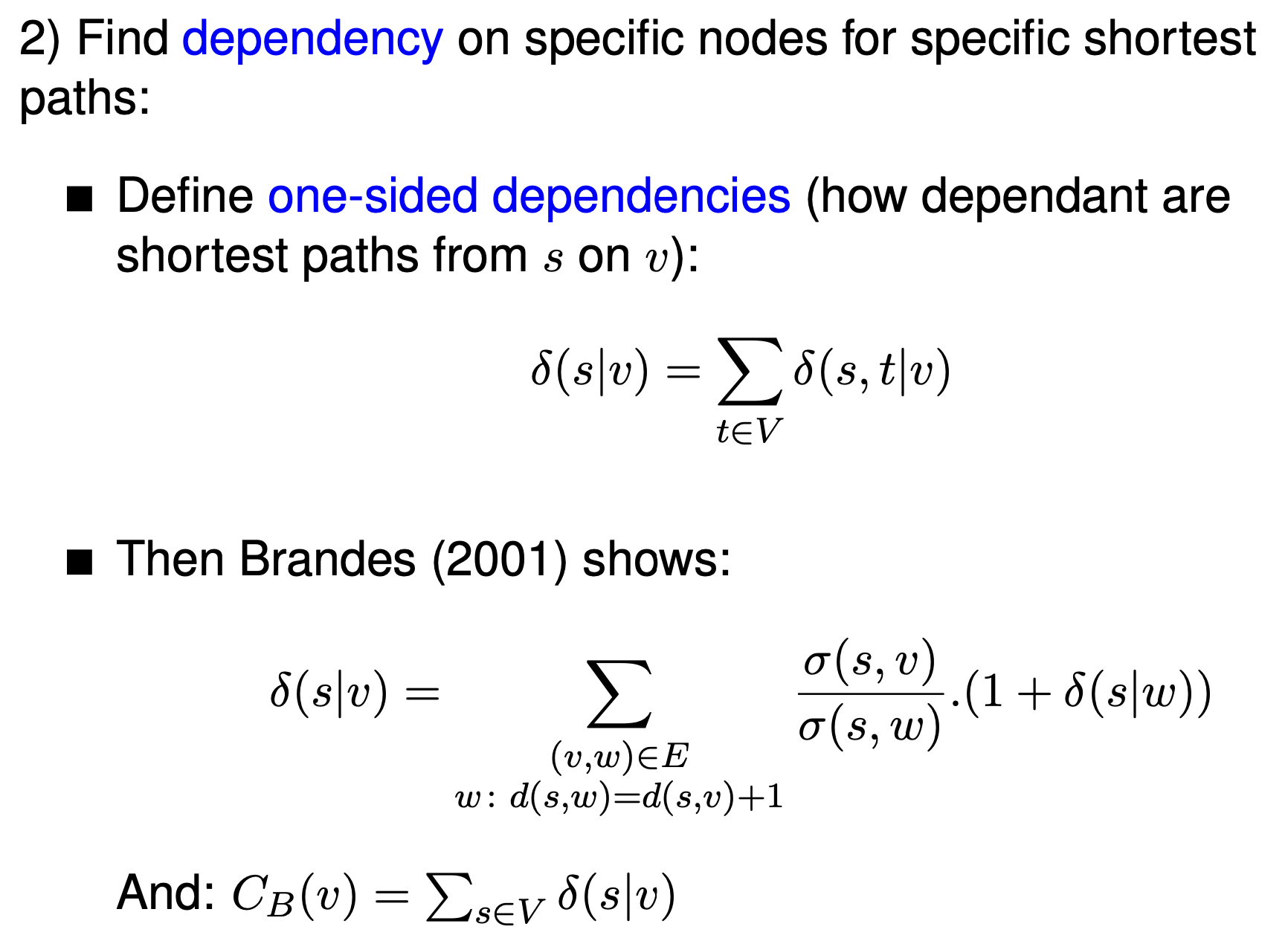
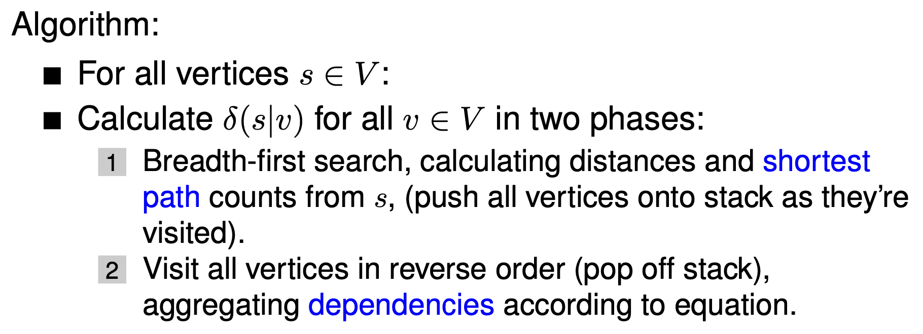
Pseudocode

Lecture 14: Clique Finding

Clustering and Classification

• Clustering: automatically grouping data according to some notion of closeness or similarity.

• Classification (e.g., sentiment classification): assigning data items to predefined classes.

• Clustering: groupings can emerge from data, unsupervised.

  • Clustering for documents, images, etc.: anything where there’s a notion of similarity between items.

• Most famous technique for hard clustering is k-means: very general (also variant for graphs).

• Also soft clustering: clusters have graded membership.

Other forms of clustering

• Agglomerative clustering works bottom-up.
• Divisive clustering works top-down, by splitting.
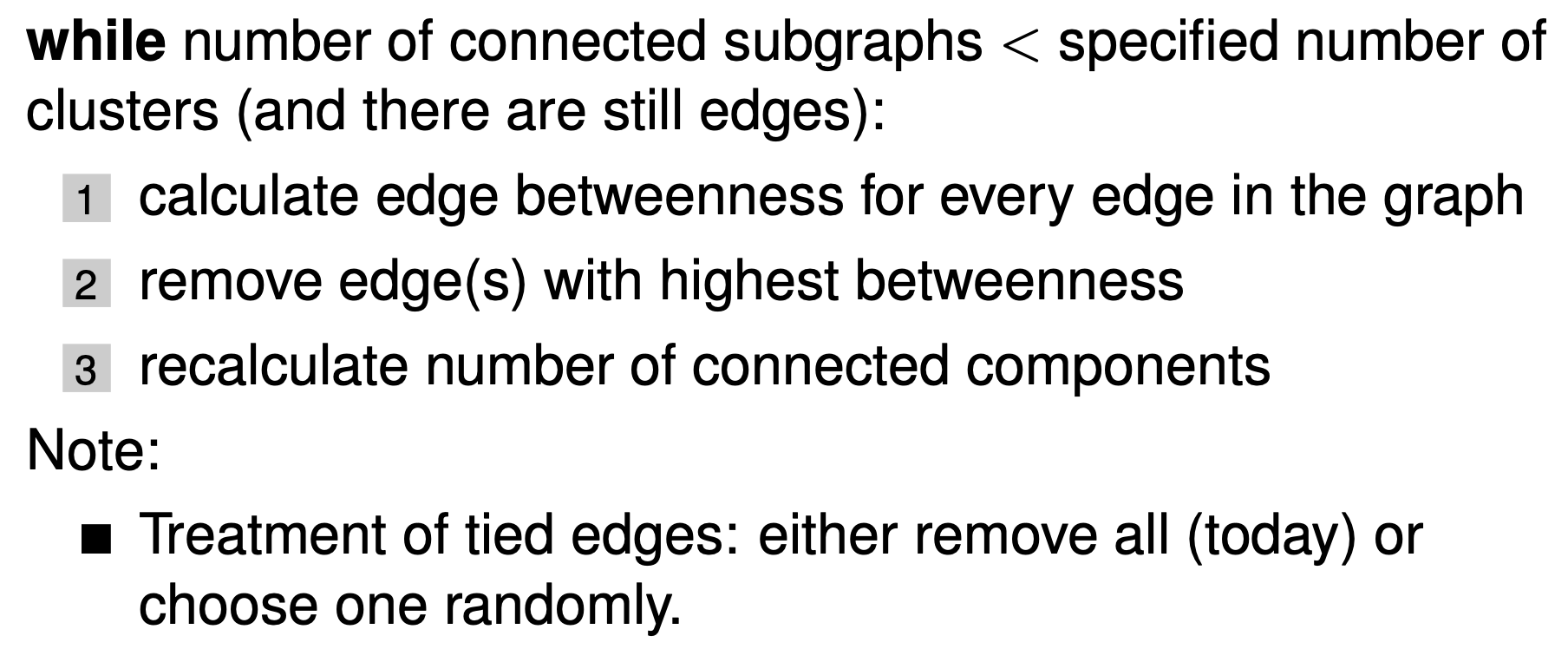
• Newman-Girvan method — a form of divisive clustering.
• Criterion for breaking links is edge betweenness centrality.

==Newman-Girvan== method

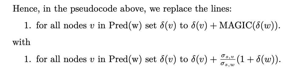
Edge betweenness centrality

• Previously: $\sigma(s, t|v)$ — the number of shortest paths between $s$ and $t$ going through node $v$.
• Now: $\sigma(s, t|e)$ — the number of shortest paths between $s$ and $t$ going through edge $e$.
• The algorithm only changes in the bottom-up (accumulation) phase:
  • $\delta(v)$ remains mostly the same.
  • $cB[(v,w)]$ is now.