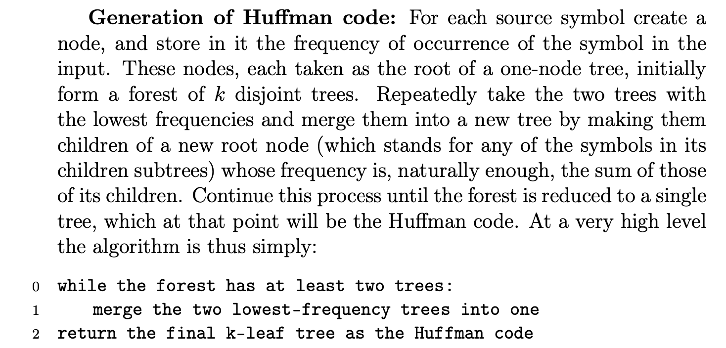
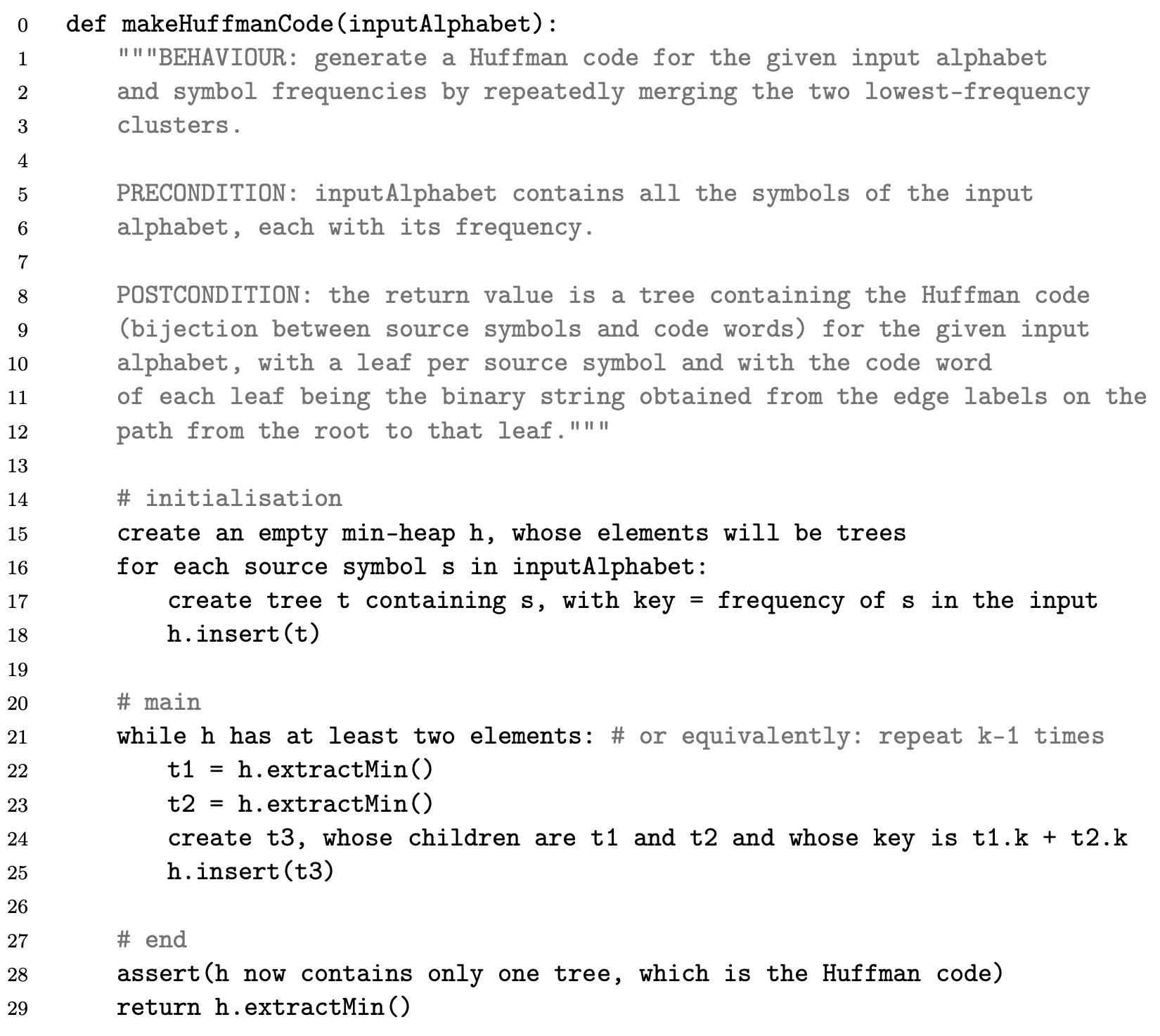
Algorithm_1And2
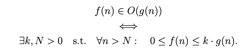
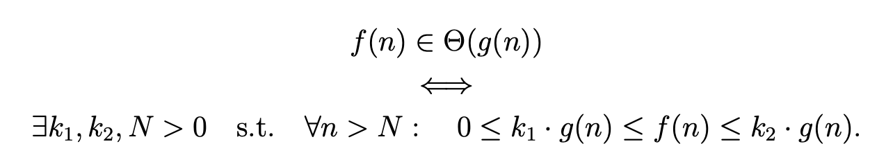
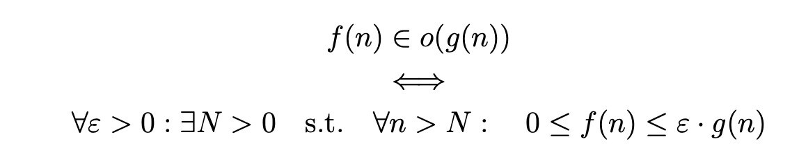
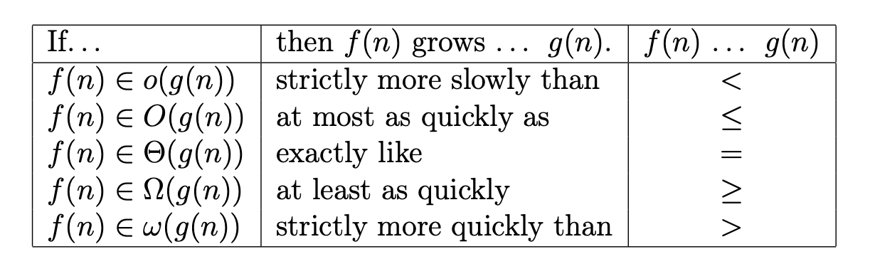
Big-O, Θ and Ω notations
Strategies
Translation strategy
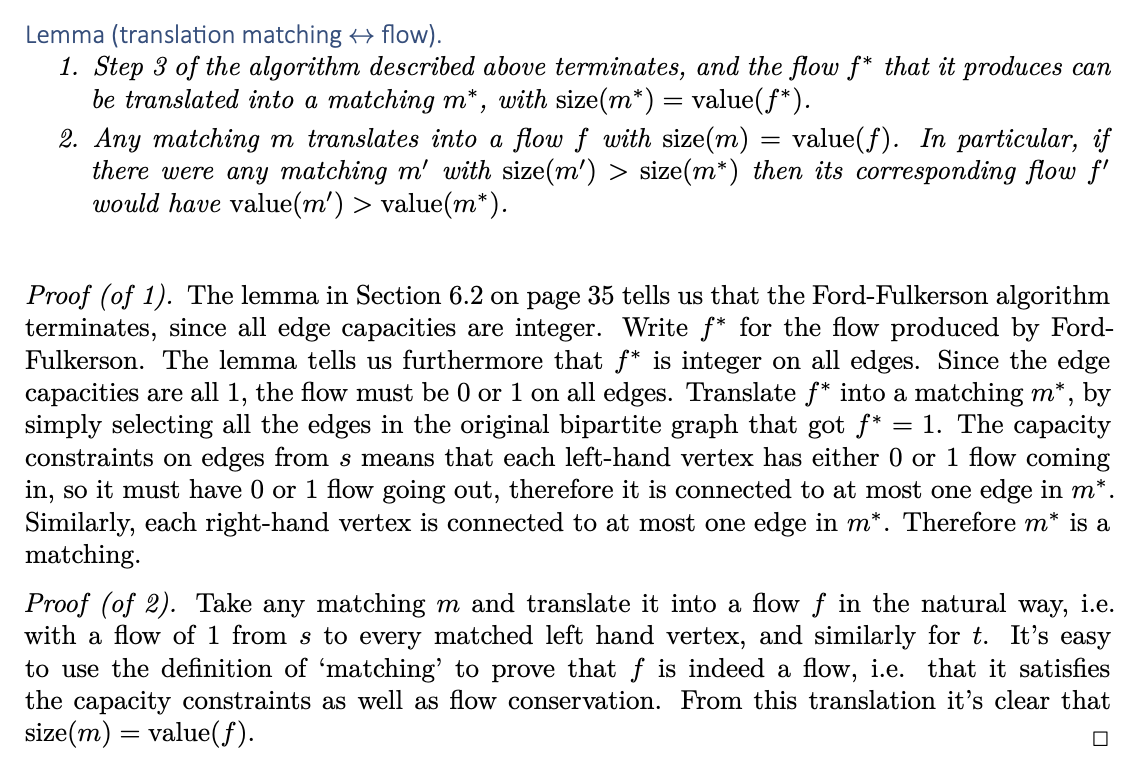
Translate the problem we want to solve into a different setting, use a standard algorithm in the different setting, then translate the answer back to the original setting. In this case, the translated setting is ‘graphs with different edge weights’. Of course we’ll need to argue why these translated answers solve the original problem.
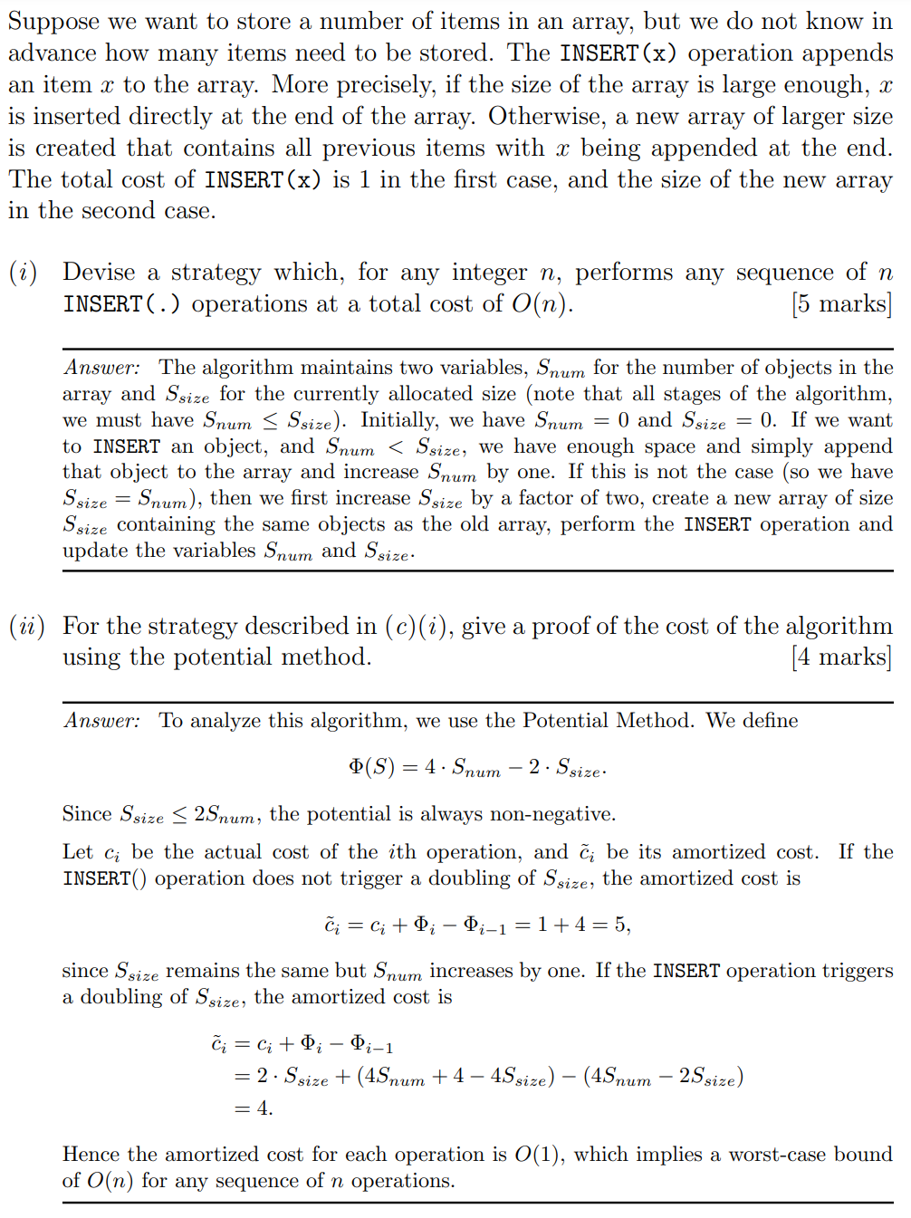
Amortized analysis
Amortized analysis is a method for calculating computational complexity, in which for any sequence of operations we ascribe an amortized cost to every operation, in such a way that the total amortized cost of a sequence of operations provides an upper bound on the actual total cost, and this upper bound is usually more representative of the actual computational cost when averaged over a large number of operations. This allows us to gain a more accurate understanding of the average performance of an algorithm over time, rather than focusing solely on the worst-case or best-case scenarios for individual operations.
Here is the formal definition. Let there be a sequence of m operations, applied to an initially-empty data structure, whose true costs are $c_1, c_2, . . . , c_m$. Suppose someone invents $c_1’,c_2’,…,c_m’$ such that (we call these amortized costs)
$$
c_1+…+c_j \le c_1’ + … c_j’ ~~~~~for ~all ~j \le m
\
\text{aggregate true cost of a sequence of operations} \le \text{ aggregate amortized cost of those operations}
$$
This is the fundamental inequality of amortized analysis
For example, we might ascribe some of the true cost of one operation A to another operation B, if A involves cleaning up some mess produced by B.
The potential method is a systematic way to choose amortized costs, as follows. We define a function $\Phi(S)$ where $S$ is a possible state of the data structure and $\Phi(S)\ge 0$, and let the amortized cost of each operation be the true cost plus the change in potential $\Delta \Phi$.
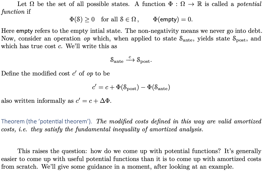
Proof of the Potential Theorem
Past papers
Define amoritized cost:
If we have a sequence of k operations whose true costs are $c_1,c_2,…c_k$, and if we devise costs $c_1’,c_2’,…,c_k’$ such that
$$
c_1+c_2+…+c_i \le c_1’ + c_2’ + … + c_i’ \text{ for all } 0\le i \le k
$$
then the $c’$ are called amortized costs
2014-p01-q09
Explain the terms amortized analysis, aggregate analysis and potential method.
In amortized analysis we consider a sequence of n data structure operations and show that the average cost of an operation is small, even though a single operation within the sequence might be very expensive.
Aggregate analysis and potential method are two techniques for performing amortized analysis. In aggregate analysis, we consider an arbitrary sequence of n operations and show an upper bound on the total cost T(n). Every operation is charged the same amortized cost, that is, the average cost T(n)/n, even though in reality some operations are cheaper or more expensive.
In the potential method, every operation may have a different amortized cost. The method overcharges cheap operations early in the sequence, storing some prepaid credit to compensate for future costly operations. The credit can be also seen as the “potential energy” stored within a data structure.
Designing Advanced Data Structures
Algorithms
Complexity
| Algorithm | Complexity |
|---|---|
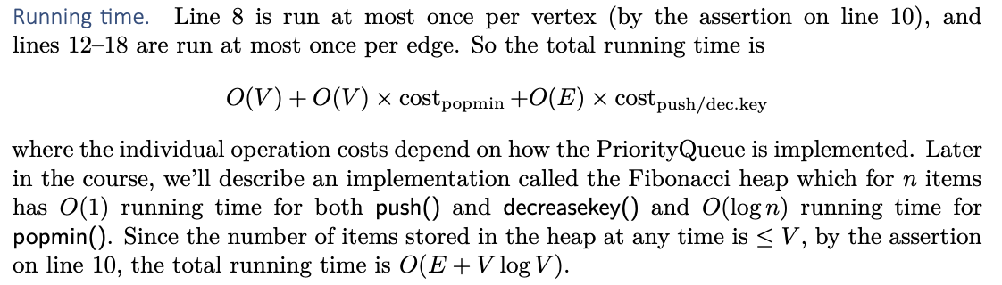
| Dijkstra | $O(E + VlogV) \text{ if all weights } \ge 0$ $=O(V ) + O(V ) × cost_{popmin} +O(E) × cost_{push/dec.key}$ |
| Bellman-Ford | $O(VE)$ |
| Prim’s algorithm | $O(E + VlogV)$ |
| Kruskal’s algorithm | $O(ElogE + E+V)=O(ElogE)=O(ElogV)$ |
| Bubble Sort | $O(N^2)$ |
| Heap Sort | $O(NlogN)$ |
| Quicksort | $O(NlogN)$ |
| Dfs_recurse_all / Dfs | $O(V+E)$ |
| Bfs | $O(V + E)$ |
| Ford Fulkerson | $O(Ef^*)$ |
| Topological sort | $O(V+E)$ |
Sorting
Minimum cost of sorting
Assertion 1 (lower bound on exchanges): If there are n items in an array, then $Θ(n)$ exchanges always suffice to put the items in order. In the worst case, $Θ(n)$ exchanges are actually needed.
Proof: Identify the smallest item present: if it is not already in the right place, one exchange moves it to the start of the array. A second exchange moves the next smallest item to place, and so on. After at worst n − 1 exchanges, the items are all in order. The bound is n − 1 rather than n because at the very last stage the biggest item has to be in its right place without need for a swap—but that level of detail is unimportant to Θ notation.
Assertion 2 (lower bound on comparisons). Sorting by pairwise comparison, assuming that all possible arrangements of the data might actually occur as input, necessarily costs at least Ω(n lg n) comparisons.
Proof: you saw in Foundations of Computer Science, there are n! permutations of n items and, in sorting, we in effect identify one of these. To discriminate between that many cases we need at least ⌈$log_2(n!)$⌉ binary tests. Stirling’s formula tells us that $n!$ is roughly $n^n$, and hence that $lg(n! )$ is about $n lg n$.
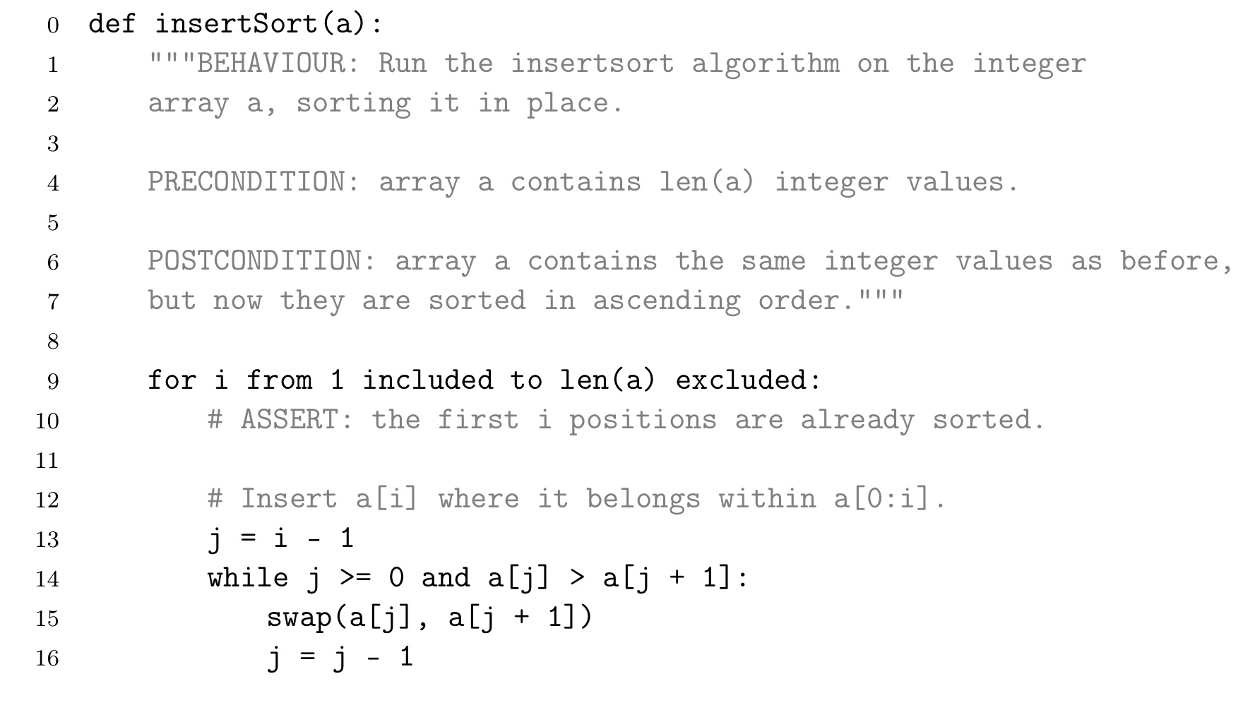
InsertSort
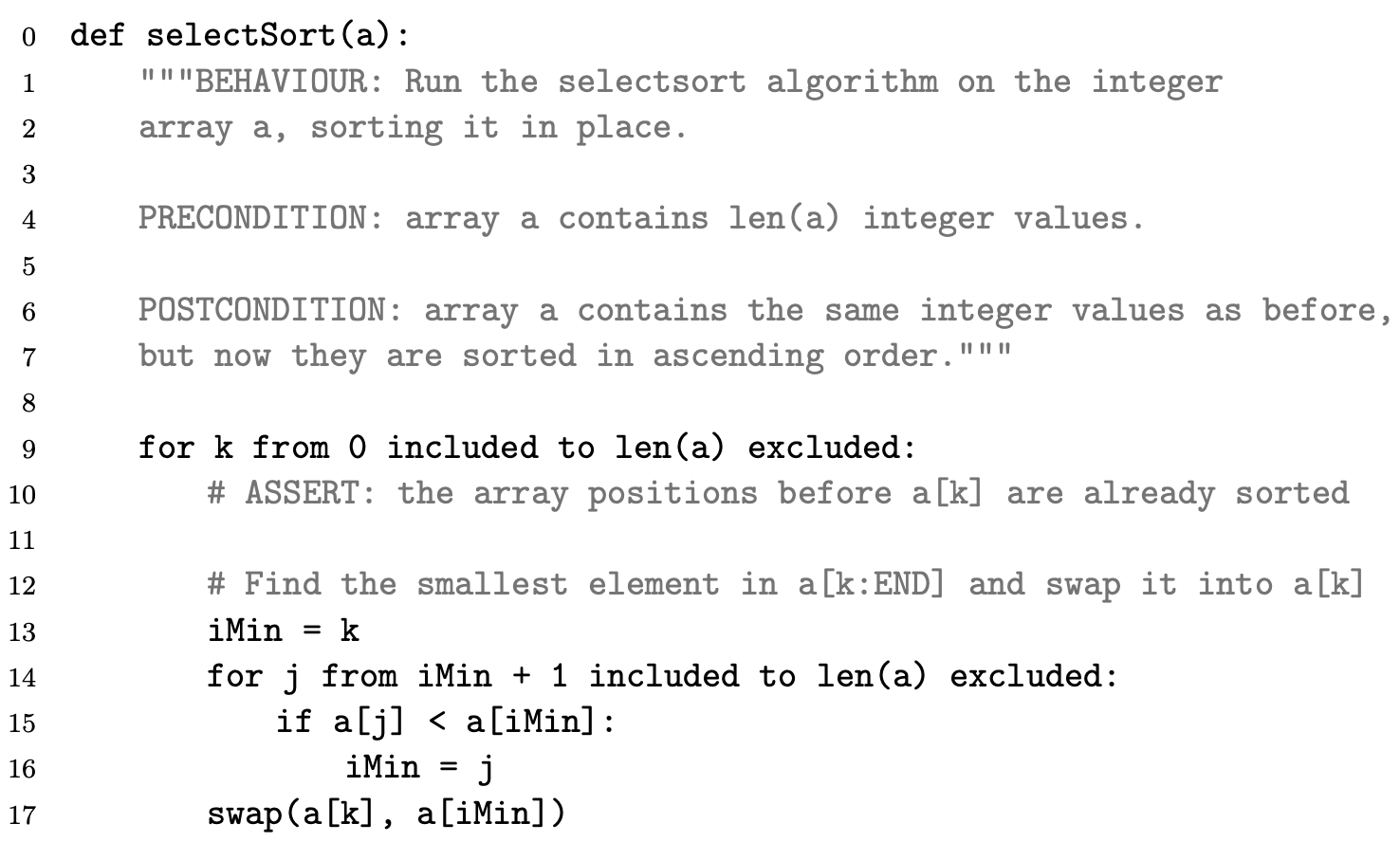
Select Sort
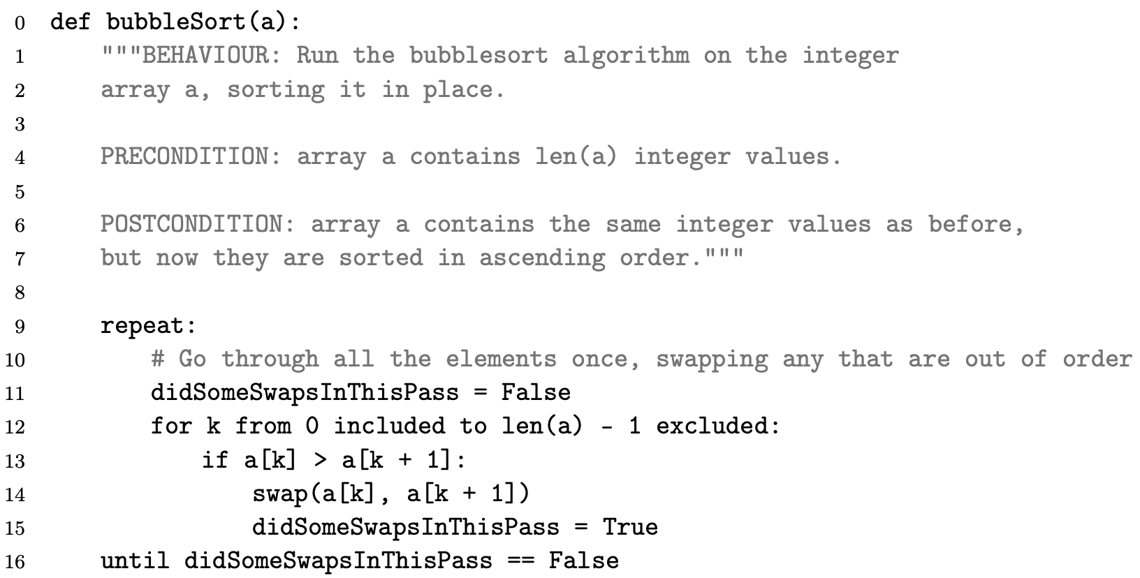
Bubble sort
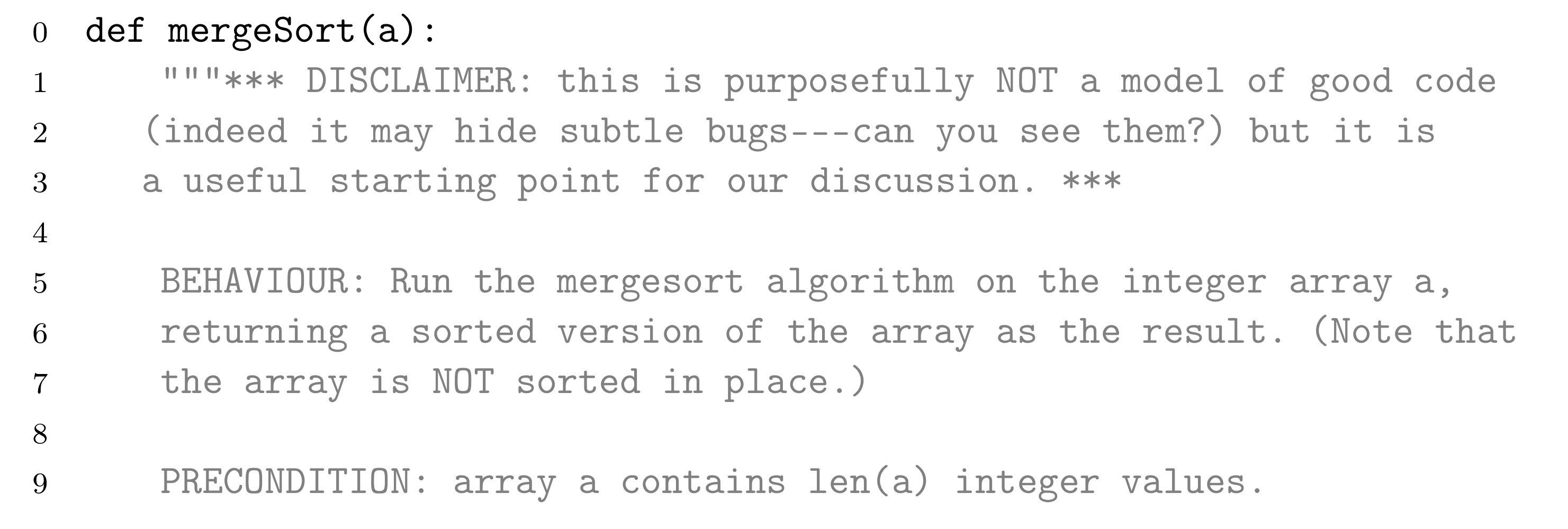
Mergesort
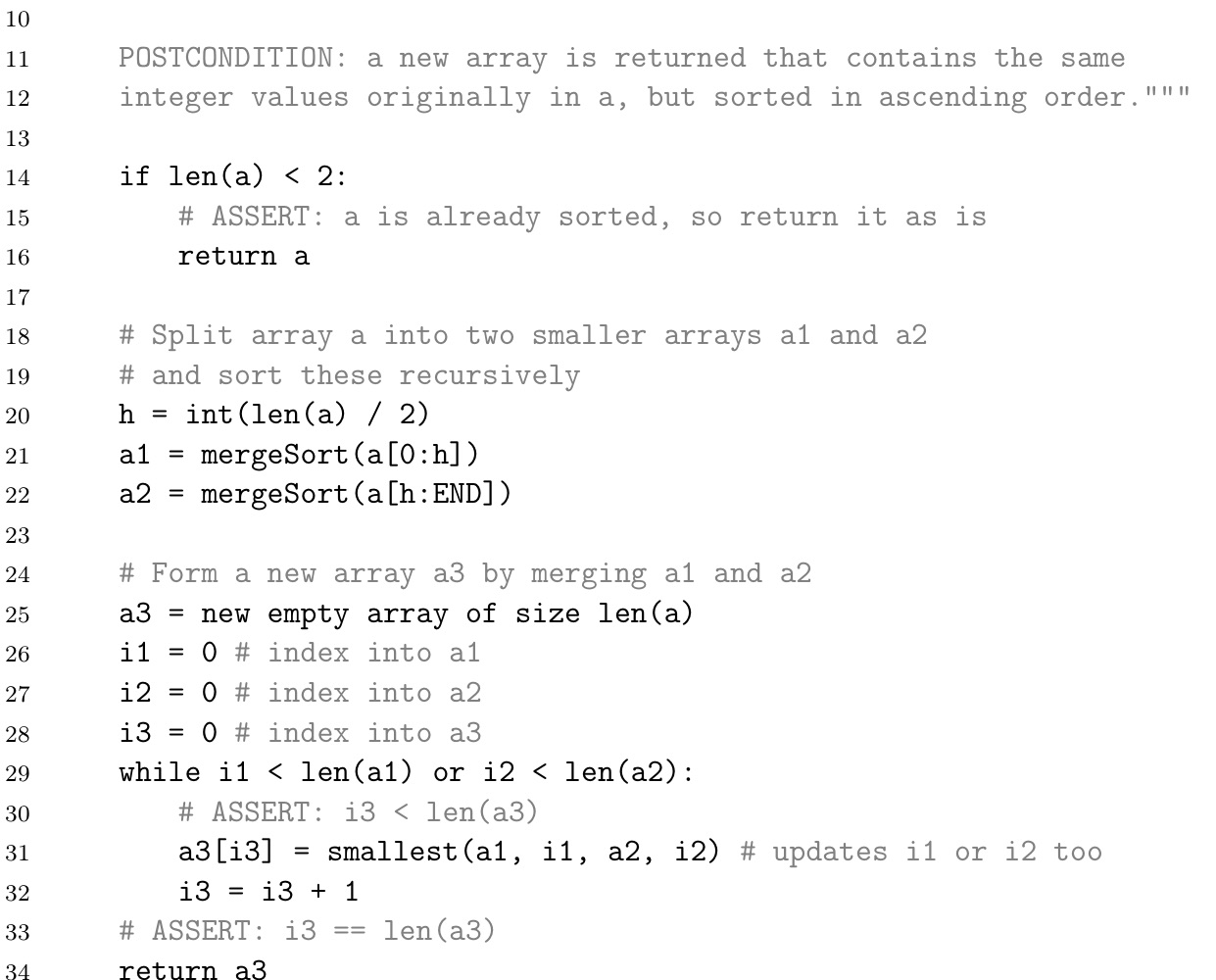
Complexity
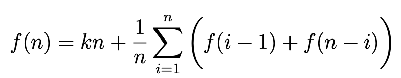
$$
f(n) = 2f(n/2)+kn \
substitution: n=2^m \
\begin{align*}
f(n)&=f(2^m)\
&=2f(2^m/2)+k2^m \
&=2f(2^{m-1})+k2^m \
&=2(2f(2^{m-2})+k2^{m-1})+k2^m \
&= 2^2f(2^{m-2})+k2^m+k2^m \
&= 2^2f(2^{m-2})+2k2^m \
&=2^3f(2^{m-3})+3k2^m \
&= … \
&= 2^mf(2^{m-m})+mk2^m\
&=f(1)\times 2^m + km2^m \
&=k_0\times 2^m + k\times m2^m \
&=k_0n + kn lgn \
&= O(nlgn)
\end{align*}
$$
Heapsort
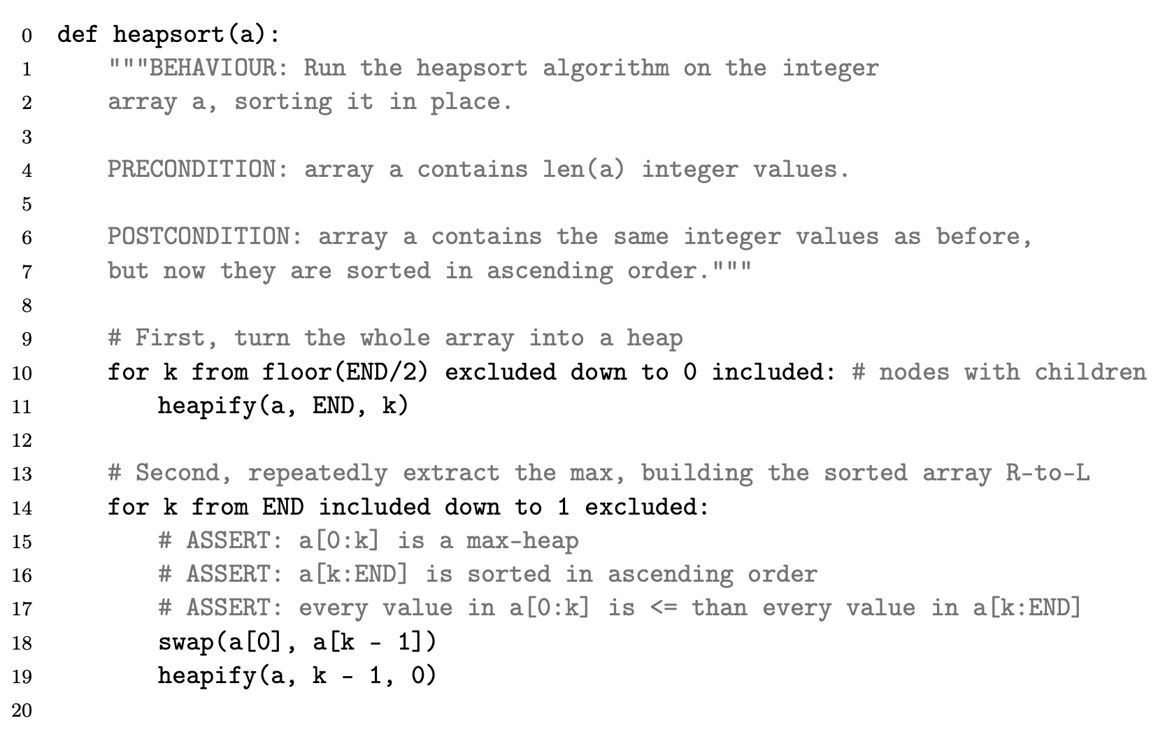
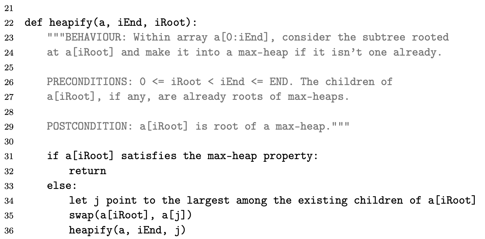
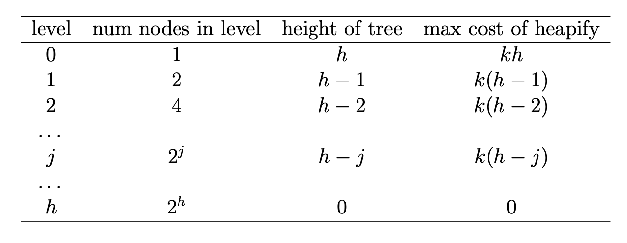
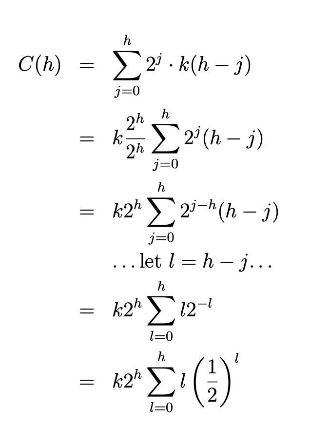
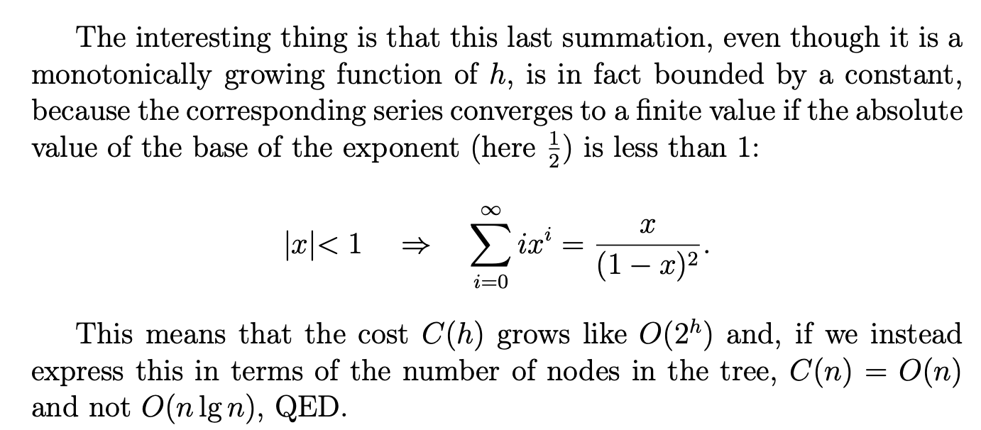
The first phase of the main heapsort function (lines 9–11) starts from the bottom of the tree (rightmost end of the array) and walks up towards the root, considering each node as the root of a potential sub- heap and rearranging it to be a heap. In fact, nodes with no children can’t possibly violate the heap property and therefore are automatically heaps; so we don’t even need to process them—that’s why we start from the midpoint floor(END/2) rather than from the end. By proceeding right-to-left we guarantee that any children of the node we are currently examining are already roots of properly formed heaps, thereby matching the precondition of heapify, which we may therefore use. It is then trivial to put an O(nlgn) bound on this phase—although, as we shall see, it is not tight.
In the second phase (lines 13–19), the array is split into two distinct parts: a[0:k] is a heap, while a[k:END] is the “tail” portion of the sorted array. The rightmost part starts empty and grows by one element at each pass until it occupies the whole array. During each pass of the loop in lines 13–19 we extract the maximum element from the root of the heap, a[0], reform the heap and then place the extracted maximum in the empty space left by the last element, a[k], which conveniently is just where it should go20. To retransform a[0:k - 1] into a heap after placing a[k - 1] in position a[0] we may call heapify, since the two subtrees of the root a[0] must still be heaps given that all that changed was the root and we started from a proper heap. For this second phase, too, it is trivial to establish an $O(nlgn)$ bound.
Heapsort therefore offers at least two significant advantages over other sorting algorithms:
- it offers an asymptotically optimal worst-case com- plexity of O(nlgn) and it sorts the array in place.
- Despite this, on non-pathological data it is still usually beaten by the amazing quicksort.
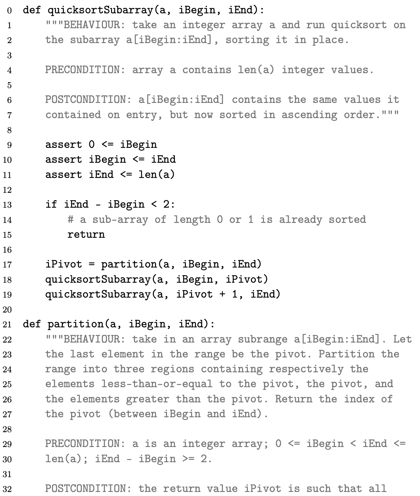
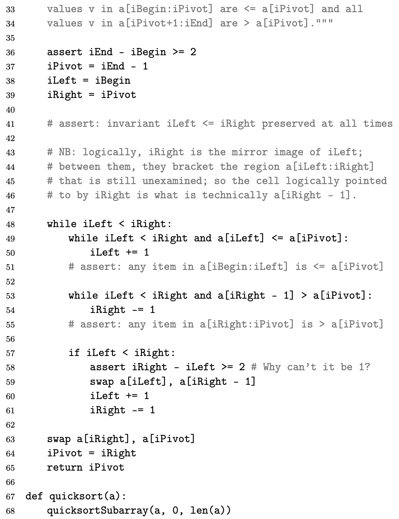
Quicksort
Average case performance
Some implementations of the Quicksort algorithm select the pivot at random, rather than taking the last entry in the input array.
- Discuss the advantages and disadvantages of such a choice.
- Quicksort has a quadratic worst case, which occurs when the result of the partioning step is maximally unbalanced in most of the recursive calls. The worst case is quite rare if the input is random but it occurs in plausible siatuation such as when the input is sorted or almost sorted. Selecting the pivot at random costs an invocation of the random number generator at every recursive call, but it makes it unlikely that the quadratic worst case will occur “naturally” with an input made of distinct values.
- How would you construct an input to trigger quadratic running time for this randomised Quicksort, without having access to the state of the random number generator?
- Make an array where all cells have the same value. Then, whatever cell is chosen as the pivot, the partition phase will put them all in the “≤” part while the “>” part will be empty, every time, leading to pessimal (quadratic) running time.
Stability of sorting methods
Data to be sorted often consists of records made of key and payload; the key is what the ordering is based upon, while the payload is some additional data that is just logically carried around in the rearranging process. In some applications one can have keys that should be considered equal, and then a simple specification of sorting might not indicate the order in which the corresponding records should end up in the output list. “Stable” sorting demands that, in such cases, the order of items in the input be preserved in the output. Some otherwise desirable sorting algorithms are not stable, and this can weigh against them.
| Sorting Algorithm | Stable/Unstable |
|---|---|
| Bubble Sort | Stable |
| Insertion Sort | Stable |
| Selection Sort | Unstable |
| Quick Sort | Unstable |
| Merge Sort | Stable |
| Heap Sort | Unstable |
| Counting Sort | Stable |
| Radix Sort | Stable |
| Bucket Sort | Stable (if implemented properly) |
Counting sort
Assume that the keys to be sorted are integers that live in a known range, and that the range is fixed regardless of the number of values to be processed. If the number of input items grows beyond the cardinality of the range, there will necessarily be duplicates in the input. If no data is involved at all beyond the integers, one can set up an array whose size is determined by the range of integers that can appear (not by the amount of data to be sorted) and initialize it to all 0s. Then, for each item in the input data, w say, the value at position w in the array is incremented. At the end, the array contains information about how many instancesof each value were present in the input, and it is easy to create a sorted output list with the correct values in it. The costs are obviously linear.
Bucket sort
Assume the input data is guaranteed to be uniformly distributed over some known range (for instance it might be real numbers in the range 0.0 to 1.0). Then a numeric calculation on the key can predict with reasonable accuracy where a value must be placed in the output. If the output array is treated somewhat like a hash table (cfr. section 4.7), and this prediction is used to insert items in it, then, apart from some local clustering effects, that data has been sorted.
To sort n keys uniformly distributed between 0.0 and 1.0, create an array of n linked lists and insert each key k to the list at position ⌊k · n⌋. This phase has linear cost. (We expect each list to be one key long on average, though some may be slightly longer and some may be empty.) In the next phase, for each entry in the array, sort the corresponding list with insertsort if it is longer than one element, then output it.
Radix Sort
Historically, radix sort was first described in the context of sorting integers encoded on punched cards, where each column of a card represented a digit by having a hole punched in the corresponding row. A mechanical device could be set to examine a particular column and distribute the cards of a deck into bins, one per digit, according to the digit in that column. Radix sort used this “primitive” to sort the whole deck.
The obvious way to proceed might seem to sort on the most significant digit, then recursively for each bin on the next significant digit, then on the next, all the way down to the least significant digit. But this would require a great deal of temporary “desk space” to hold the partial mini- decks still to be processed without mixing them up.
Radix sort instead proceeds, counter-intuitively, from the least significant digit upwards. First, the deck is sorted into b = 10 bins based on the least significant digit. Then the contents of the bins are collected together, in order, to reform a full deck, and this is then sorted according to the next digit up. But the per-digit sorting method used is chosen to be stable, so that cards that have the same second digit still maintain their relative order, which was induced by the first (least significant) digit. The procedure is repeated going upwards towards the most significant digits. Before starting pass i, the digits in positions 0 to i − 1 have already been sorted. During pass i, the deck is sorted on the digit in position i, but all the cards with the same i digit remain in the relative order determined by the even less significant digits to their right. The result is that, once the deck has been sorted on the most significant digit, it is fully sorted. The number of passes is equal to the number of digits (d) in the numerals being sorted and the cost of each pass can be made linear by using counting sort.
The number of passes is equal to the number of digits (d) in the numerals being sorted and the cost of each pass can be made linear by using counting sort
Explain how radix sort works, to what inputs it can be applied and what its asymptotic complexity is.
Radix sort was invented in the context of sorting punched cards. It is a linear-time algorithm for sorting an arbitrary number of strings of fixed (or, more precisely, bounded) length over a small alphabet. It uses as a subroutine a stable linear-time sorting algorithm for items consisting of a single character over the given alphabet, such as for example counting sort.
Assume the strings have maximum length l and that shorter strings are right-padded with blanks or left-padded with zeros in case of strings of digits—whatever is appropriate for the desired sorting order.
Consider the character positions from the least significant (rightmost, index 0) to the most significant (leftmost, index l − 1). For each character position i, use a linear-time stable sort to sort all the strings based on the character at that position.
The main loop runs l times. Each run is one invocation of a linear-time stable sort. Thus the whole algorithm takes O(nl) which, if l is taken as a constant, is O(n).
Explain why running radix sort does not proceed from most to least significant digit, as would at first seem more intuitive.
It might feel more natural to sort first by most significant digit (or character position), because then each of the intermediate passes would bring the individual elements closer and closer to their intended position. However the subsequent passes would have to act separately on each of the “bins” of equal-value characters found in the previous pass, thus requiring additional storage space and possibly a recursive arrangement—both inconvenient in the context of sorting physical punched cards.
By running in the opposite direction instead, i.e. from least to most significant character position, while it’s true that the intermediate passes may appear to “jumble up” the list of items as they go, each pass can run simply on the whole result of the previous one, without requiring recursion nor any additional space beyond that required by the stable sort used as a subroutine.
Dynamic programming
Explain the programming technique known as memoization, detailing the cases to which it applies
Memoization is a time-space trade-off (1) technique in which previously computed results are remembered instead of being recomputed (1). A table that survives between invocations of the function is indexed by the tuple of arguments (1) that the function expects. Before computing a value, the function first checks whether a result for that tuple of input arguments is already present in the table. If so, the previously computed value is returned in constant time (1). This technique is particularly effective when applied to recursive functions that recompute the same partial results over and over again (1), as happens for example in top-down dynamic programming (1). (Earn marks as indicated, up to a maximum of 4.)
Write a memoized recursive function to compute the ith Fibonacci number F(i)
1 | function fib(i): |
Matrix chain multiplication
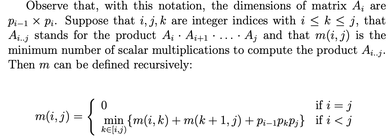
1 | function matrix_chain_order(p) |
Longest common subsequence
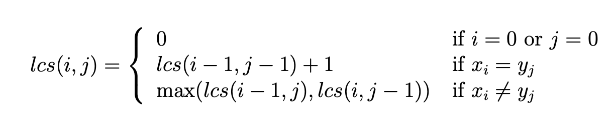
1 | function LCS(X[1..m], Y[1..n]) |
Greedy Algorithms
Explain the greedy strategy in algorithm design. To what problems does it apply?
The greedy strategy applies to problems made of overlapping subproblems with optimal substructure, like dynamic programming. The greedy strategy, however, does not at every stage compute the optimal solution for all possible choices of a parameter; instead, it selects the best-looking choice a priori and proceeds to find an optimal solution for the remaining subproblem.
In order to ensure that the globally optimal solution will be found, it is necessary to prove that the “best-looking choice” is indeed part of an optimal solution. If this proof is missing, the answer given by the greedy algorithm may in fact be wrong
If a problem can be solved with both dynamic programming and a greedy algorithm, what are the advantages of using one or the other?
Almost all problems that can be solved by a greedy algorithm can also be solved by dynamic programming (though not vice versa). When both approaches work, the greedy one is usually more efficient and should be preferred. The dynamic programming solution however does not require developing a heuristic for finding the best choice, nor a proof (sometimes rather hard to develop) that the choice picked by the heuristic is actually part of a globally optimal solution.
Activity Scheduling
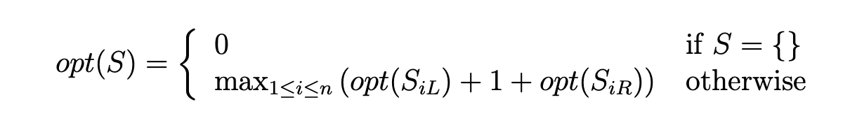
DP version
Greedy version
In this example the greedy strategy is to pick the activity that finishes first, based on the intuition that it’s the one that leaves most of the rest of the timeline free for the allocation of other activities. Now, to be able to use the greedy strategy safely on this problem, we must prove that this choice is indeed optimal; in other words, that the ai ∈ S with the smallest fi is included in an optimal solution for S. That activity would be the lowest-numbered ai in S, by the way, or a1 at the top level, since we conveniently stipulated that activities were numbered in order of increasing finishing time.
Proof by contradiction. Assume there exists an optimal solution O ⊂ S that does not include a1. Let ax be the activity in O with the earliest finishing time. Since a1 had the smallest finishing time in all S, f1 ≤ fx. There are two cases: either f1 ≤ sx or f1 > sx. In the first case, s1 < f1 ≤ sx < fx, we have that a1 and ax are disjoint and therefore compatible, so we could build a better solution than O by adding a1 to it; so this case cannot happen. We are left with the second case, in which there is overlap because a1 finishes after ax starts (but before ax finishes, by hypothesis that a1 is first to finish in S). Since ax is first to finish in O and no two activities in O overlap, then no activity in O occurs before ax, thus no activity in O (aside from ax) overlaps with a1. Thus we could build another equally good optimal solution by substituting a1 for ax in O. Therefore there will always exist an optimal solution that includes a1, QED.
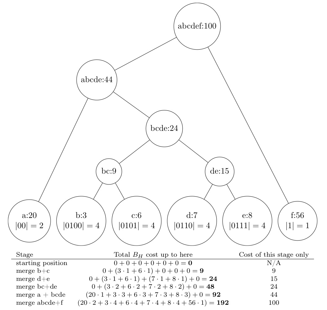
Huffman codes
Data structures
Complexities
| Data Structure | Insertion/Push | Deletion | Search | Extract Minimum/Maximum | Successor/Predecessor | DecreaseKey | Merge |
|---|---|---|---|---|---|---|---|
| Fibonacci Heap | $O(1)$ | $O(logN)$ | O(1) | ||||
| Linked list heap | $O(1)$ | $O(logN)$ | |||||
| Binary heap | $O(logN)$ | $O(logN)$ | |||||
| Binomial heap | $O(logN)$ | $O(logN)$ | $O(logN)$ | $O(logN)$ | $O(logN)$ | ||
| Binary Search Tree | $O(logN)$ | $O(logN)$ | $O(logN)$ | $O(logN)$ | |||
| Red Black Tree | $O(logN)$ | $O(logN)$ | $O(logN)$ |
Abstract Data Type
List
Lists provide one natural implementation of stacks, and are the data structure of choice in many places where flexible representation of variable amount of data is wanted.
Doubly-linked list
A feature of lists is that, from one item, you can progress along the list in one direction very easily; but once you have taken the next of a list, there is no way of returning. To make it possible to traverse a list in both directions one might define a new type called Doubly Linked List in which each wagon had both a next and a previous pointer.
$$
w.next.previous == w
$$
Equation (1) would hold for every wagon inside the DLL except for the last
$$
w.previous.next == w
$$
Euqation (2) would hold for every wagon inside the DLL except for the first.
Graph representation (using List)
Represent each vertex by an integer, and having a vector such that element $i$ in the vector holds the head of a list of all the vertices connected directly to edges radiating from vertex $i$.
ADT List
1 | ADT List { |
Stack
- LIFO (last in first out)
1 | ADT Stack { |
Implementations
- Combination of an array and an index (pointing to the “top of stack”)
- The
pushoperation writes a value into the array and increments the index - The
popoperation delets a value from the array and decrements the index
- The
- Linked lists
- Pushing an item adds an extra cell to the front of a list
- Popping removes the cell at the front of the list
Use cases
- Reverse Polish Notation (e.g.
3 12 add 4 mul 2 sub->(3 x 12) x 4 - 2)
Queue and Deque
- FIFO (first in first out)
1 | ADT Queue{ |
1 | ADT Queue{ |
Dictionary
- Also known as Maps, Tables, Associative arrays, or Symbol tables
1 | ADT Dictionary { |
Set
1 | boolean isEmpty(); |
Binary Search Tree
To find the successor s of a node x whose key is kx, look in x’s right subtree: if that subtree exists, the successor node s must be in it—otherwise any node in that subtree would have a key between kx and ks, which contradicts the hypothesis that s is the successor. If the right subtree does not exist, the successor may be higher up in the tree. Go up to the parent, then grand-parent, then great-grandparent and so on until the link goes up-and-right rather than up-and-left, and you will find the successor. If you reach the root before having gone up-and-right, then the node has no successor: its key is the highest in the tree.
2-3-4 trees
A 2-3-4 tree is a type of balanced search tree where every internal node can have either 2, 3, or 4 children, hence the name. More specifically:
A 2-node has one data element, and if it is not a leaf, it has two children. The elements in the left subtree are less than the node’s element, and the elements in the right subtree are greater.
A 3-node has two data elements, and if it is not a leaf, it has three children. The elements in the left subtree are less than the first (smaller) element in the node, the elements in the middle subtree are between the node’s elements, and the elements in the right subtree are greater than the second (larger) element.
A 4-node has three data elements, and if it is not a leaf, it has four children. The elements in the first (leftmost) subtree are less than the first (smallest) element in the node, the elements in the second subtree are between the first and second elements in the node, the elements in the third subtree are between the second and third elements in the node, and the elements in the fourth (rightmost) subtree are greater than the third (largest) element.
The key property of a 2-3-4 tree is that all leaf nodes are at the same depth, which ensures the tree remains balanced and operations such as insertion, deletion, and search can be performed in logarithmic time.
2-3-4 trees are commonly used in the implementation of databases and file systems. They are a type of B-tree, and in fact, the widely used B-tree and B+ tree structures are generalizations of 2-3-4 trees.
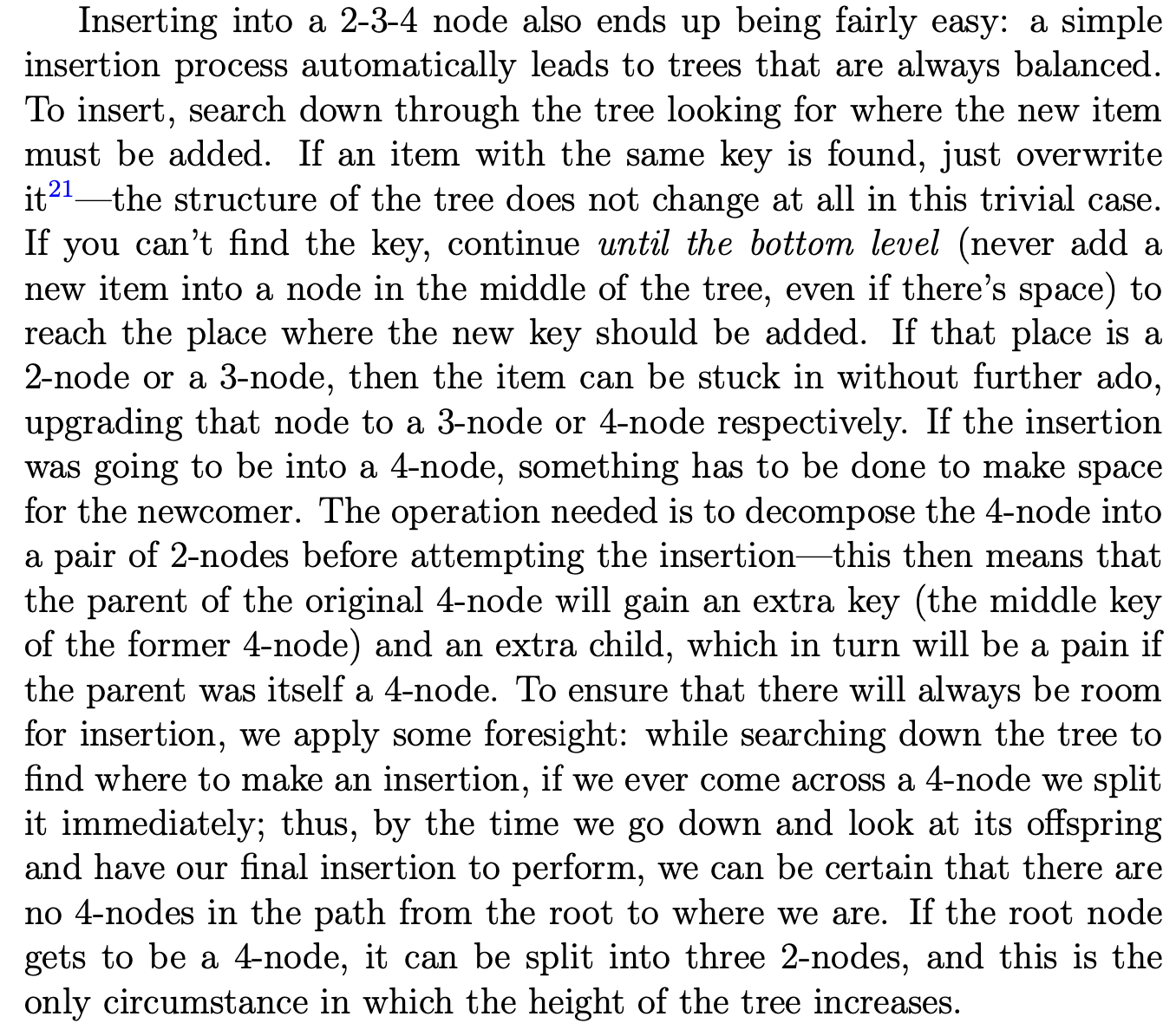
Inserting
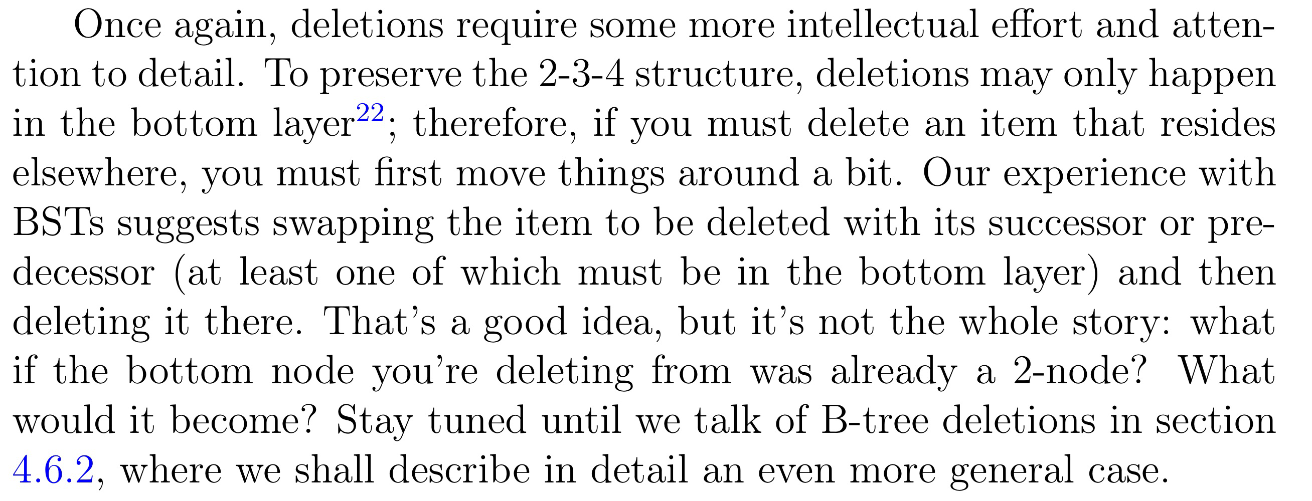
Deletion
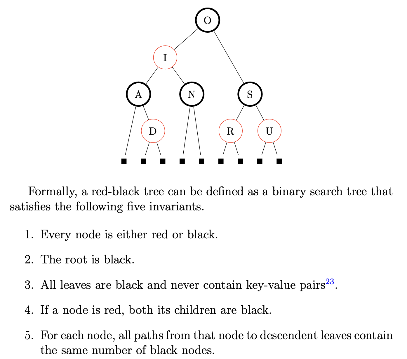
Red-black trees
Rotations
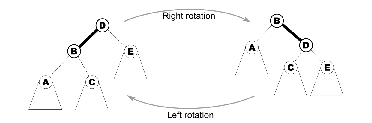
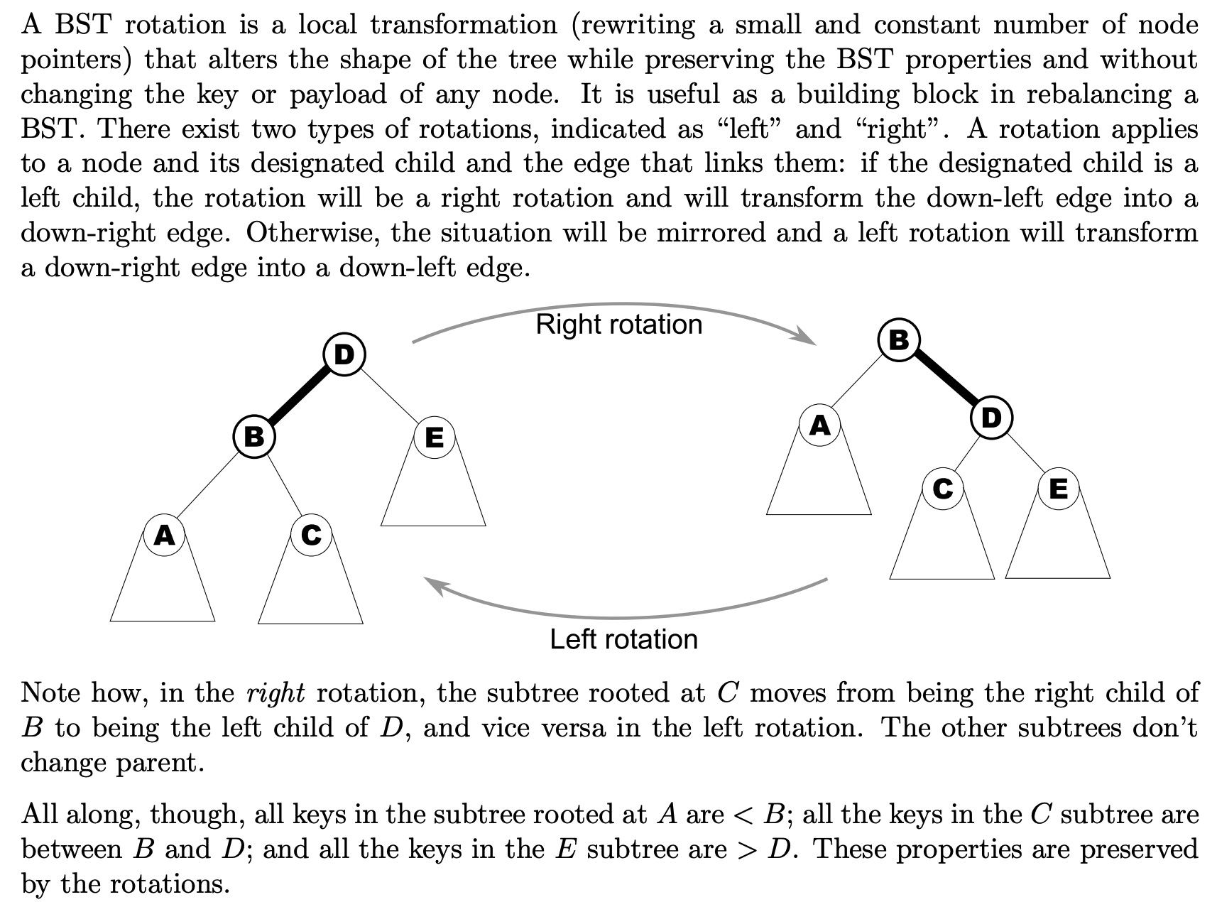
What is a BST rotation
2014-p01-q08
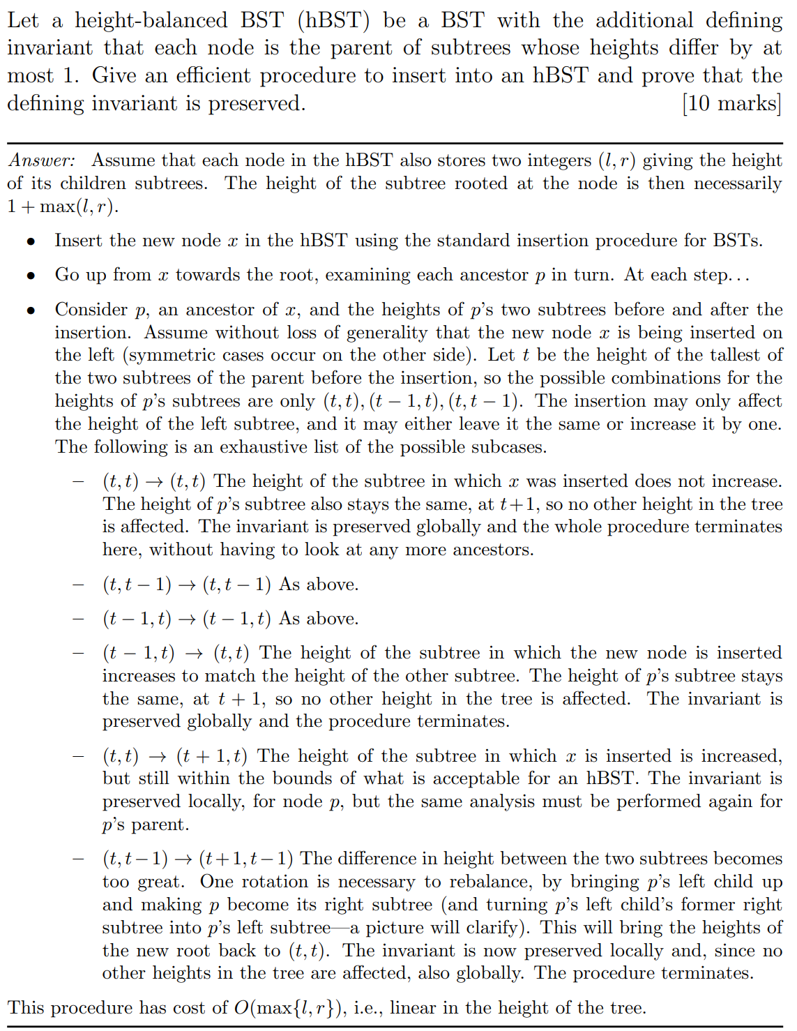
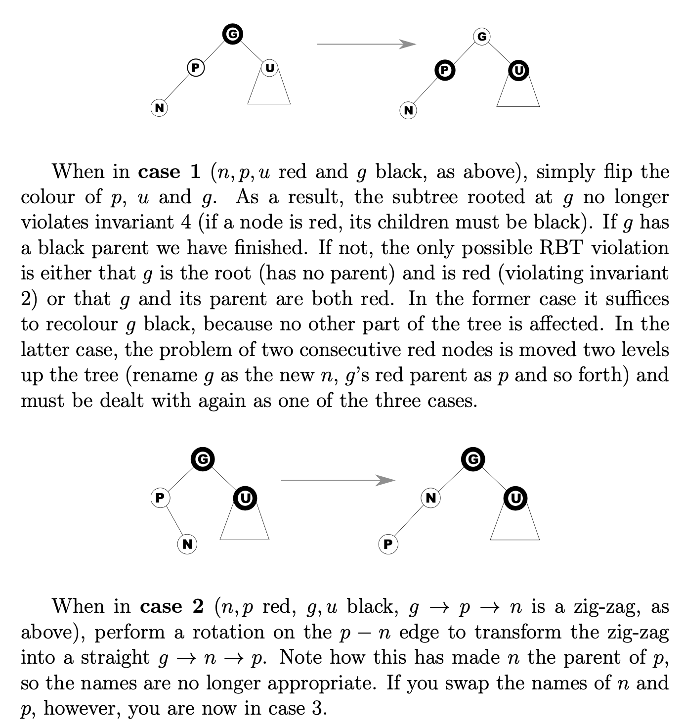
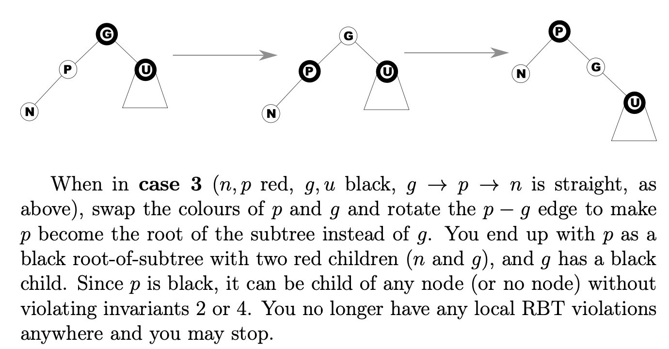
Insertion
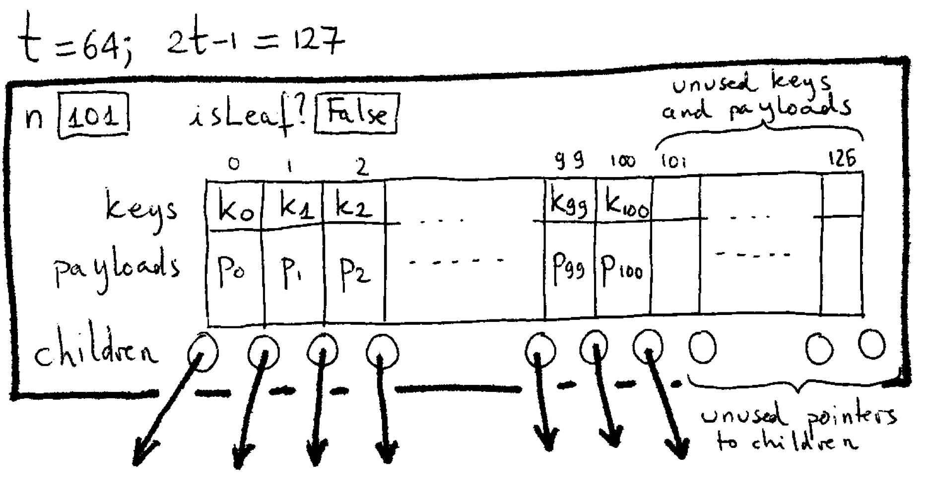
B-Trees
Rules
- There are internal nodes (with keys and payloads and children) and leaf nodes (without keys or payloads or children).
- For each key in a node, the node also holds the associated payload.
- All leaf nodes are at the same distance from the root.
- All internal nodes have at most 2t children; all internal nodes except the root have at least t children.
- A node has c children iff it has c−1 keys.
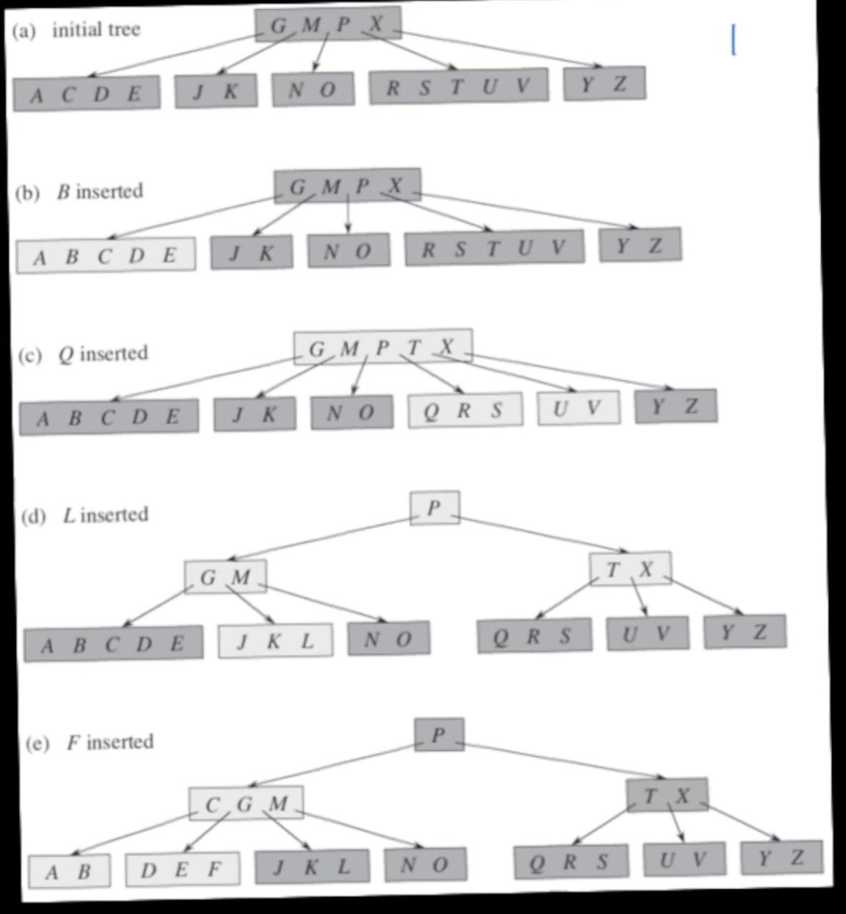
Inserting
To insert a new key (and payload) into a B-tree, look for the key in the B-tree in the usual way. If found, update the payload in place. If not found, you’ll be by then in the right place at the bottom level of the tree (the one where nodes have keyless leaves as children); on the way down, whenever you find a full node, split it in two on the median key and migrate the median key and resulting two children to the parent node (which by inductive hypothesis won’t be full). If the root is full when you start, split it into three nodes (yielding a new root with only one key and adding one level to the tree). Once you get to the appropriate bottom level node, which won’t be full or you would have split it on your way there, insert there.
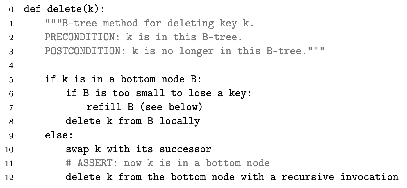
Deleting
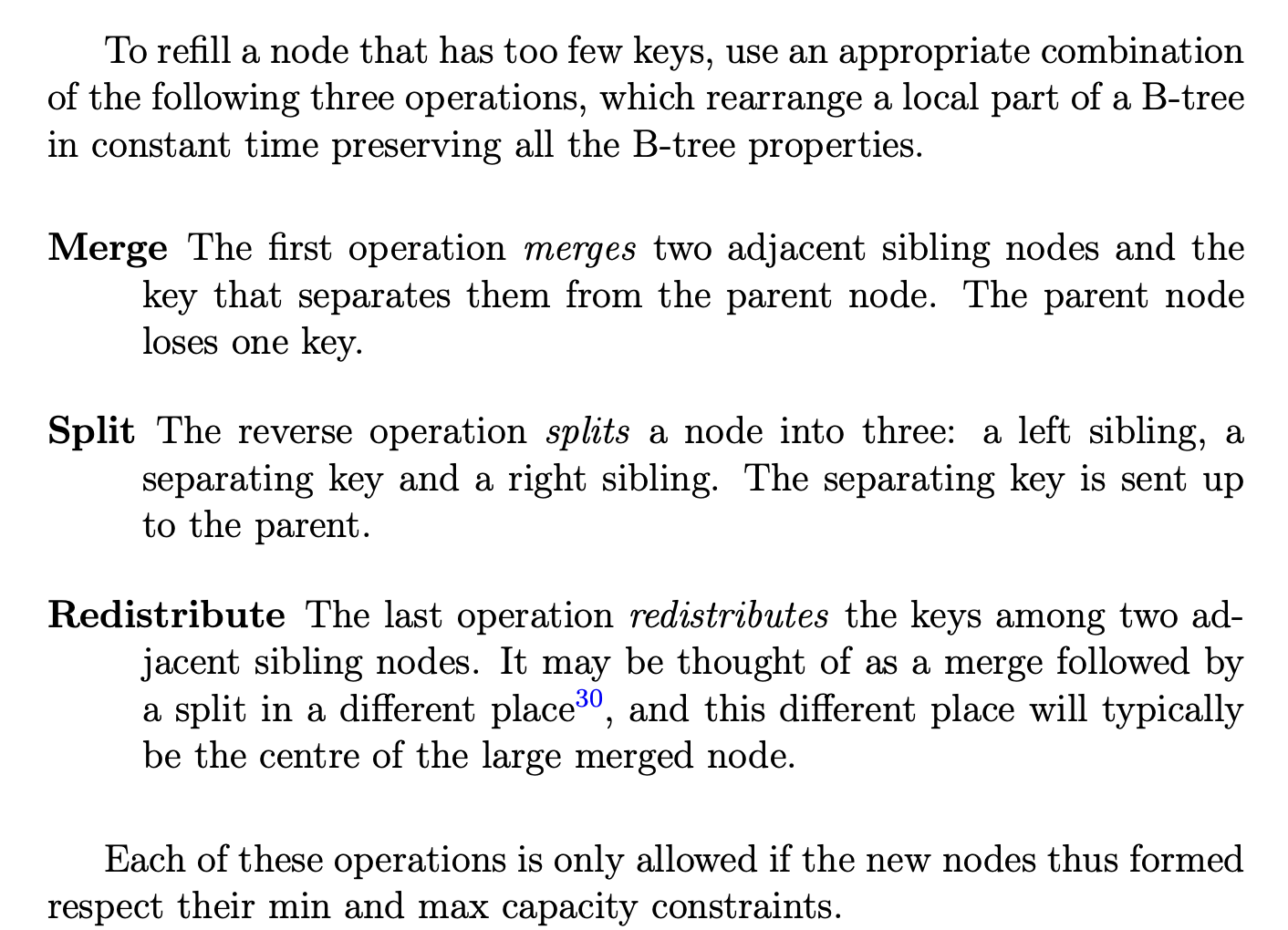
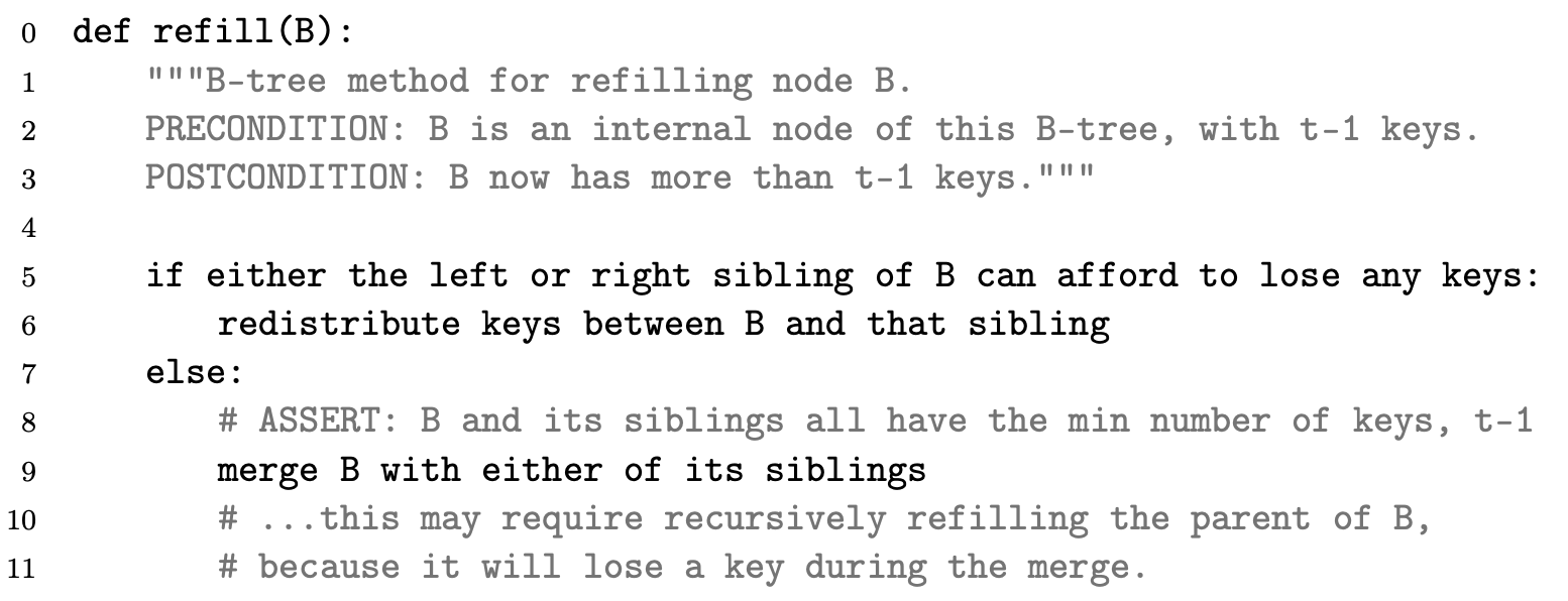
Deleting is a more elaborate affair because it involves numerous subcases. You can’t delete a key from anywhere other than a bottom node (i.e. one whose children are keyless leaves), otherwise you upset its left and right children that lose their separator. In addition, you can’t delete a key from a node that already has the minimum number of keys. So the general algorithm consists of creating the right conditions and then deleting (or, alternatively, deleting and then readjusting).
To move a key to a bottom node for the purpose of deleting it, swap it with its successor (which must be in a bottom node). The tree will have a temporary inversion, but that will disappear as soon as the unwanted key is deleted.
Refill
Hash table
Briefly explain hash functions, hash tables, and collisions
A hash function is a mapping from a key space (for example strings of characters) to an index space (for example the integers from 0 to m-1).
A hash table is a data structure that stores (key,value) pairs indexed by unique key. It offers efficient (typically O(1)) access to the pair, given the key. The core idea is to store the pairs in an array of m elements, placing each pair in the array position given by the hash of the key.
Since the key space is potentially much larger than the index space, the hash function will necessarily map several keys to the same slot. This is known as a collision. Some scheme must be adopted to resolve collisions, other wise the hash table can’t work. The two main strategies involving either storing the colliding pairs in a linked list external to the table (chaining) or storing colliding pairs within the table but at some other position.
Chaining
We can arrange that the locations in the array hold little linear lists that collect all the keys that hash to that particular value. A good hash function will distribute keys fairly evenly over the array, so with luck this will lead to lists with average length ⌈n/m⌉ if n keys are in use.
Open addressing
The second way of using hashing is to use the hash value h(n) as just a first preference for where to store the given key in the array. On adding a new key, if that location is empty then well and good—it can be used; otherwise, a succession of other probes are made of the hash table according to some rule until either the key is found to be present or an empty slot for it is located. The simplest (but not the best) method of collision resolution is to try successive array locations on from the place of the first probe, wrapping round at the end of the array34. Note that, with the open addressing strategy, where all keys are kept in the array, the array may become full, and that its performance decreases significantly when it is nearly full; implementations will typically double the size of the array once occupancy goes above a certain threshold.
Linear probing
This easy probing function just returns $h(k) + j \mod m.$ In other words, at every new attempt, try the next cell in sequence. It is always a permutation. Linear probing is simple to understand and implement but it leads to primary clustering: many failed attempts hit the same slot and spill over to the same follow-up slots. The result is longer and longer runs of occupied slots, increasing search time.
Quadratic probing
With quadratic probing you return $h(k) + cj + dj^2 \mod m$ for some constants c and d. This works much better than linear probing, provided that c and d are chosen appropriately: when two distinct probing sequences hit the same slot, in subsequent probes they then hit different slots. However it still leads to secondary clustering because any two keys that hash to the same value will yield the same probing sequence.
Double hashing
With double hashing the probing sequence is $h1(k)+ j · h2(k) \mod m$, using two different hash functions h1 and h2. As a consequence, even keys that hash to the same value (under h1) are in fact assigned different probing sequences. It is the best of the three methods in terms of spreading the probes across all slots, but of course each access costs an extra hash function computation.
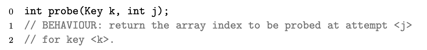
Explain the open addressing strategy of collision resolution and the term probing sequence used in that context.
The open addressing strategy resolves collisions by allowing several successive probes for the same key, with each probe generating a new position to be tried. The sequence of indices generated by a given key is called the probing sequence for that key.
Explain quadratic probing and its advantages and disadvantages. [Hint: refer to primary and secondary clustering.
In quadratic probing, the probing function is a quadratic polynomial of the probe number. This has the advantage of avoiding the primary clustering problem of the simpler linear probing strategy in which, whenever the probing sequence for a key $k_1$ contains the value of h($k_2$) for some other key $k_2$, the two probing sequences collide on every successive value from then onwards, causing a vicious circle of more and more collisions. With quadratic probing, the sequences may collide in that position, but will then diverage again for subsequent probes, However, quadratic probing still stuffers from secondary clustering: if two distinct keys hash to the same value, their probing sequences will be identical and will collide at every probe number.
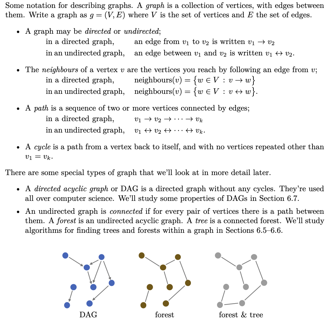
Graphs and path finding
Notation and representation
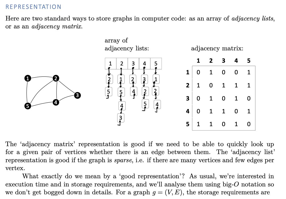
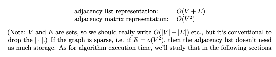
Consider the two standard representations of directed graphs: the adjacency-list representation and the adjacency-matrix representation. Find a problem that can be solved more efficiently in the adjacency-list representation than in the adjacency-matrix representation, and another problem that can be solved more efficiently in the adjacency-matrix representation than in the adjacency-list representation.
Problem 1: Is there an edge from node u to v? In the adjacency-matrix representation, we can quickly test this by looking up the entry $a_{u,v}$ of the adjacency matrix, which takes $O(1)$ time. In the adjacency list representation, we may need to go through the whole list $Adj[u]$ which might take $\theta(V)$ time
Problem 2: Is the node u a sink (i.e., are there any outgoing edges from u)? In the adjacency-list representation we can test in $O(1)$ time whether a node u is a sink by checking whether the list $Adj[u]$ is empty or not. In the adjacency-matrix representation, however, this requires $\theta(V)$ time
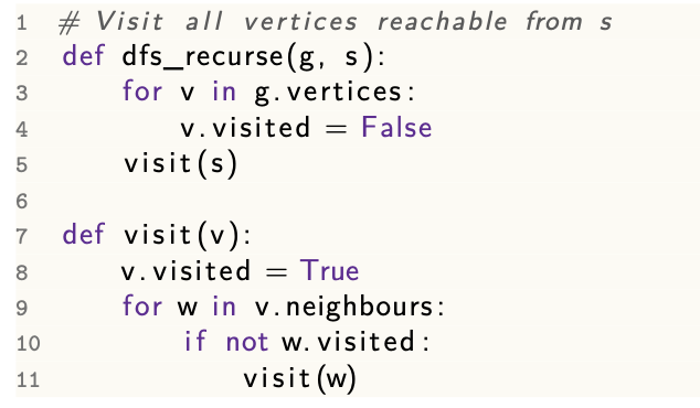
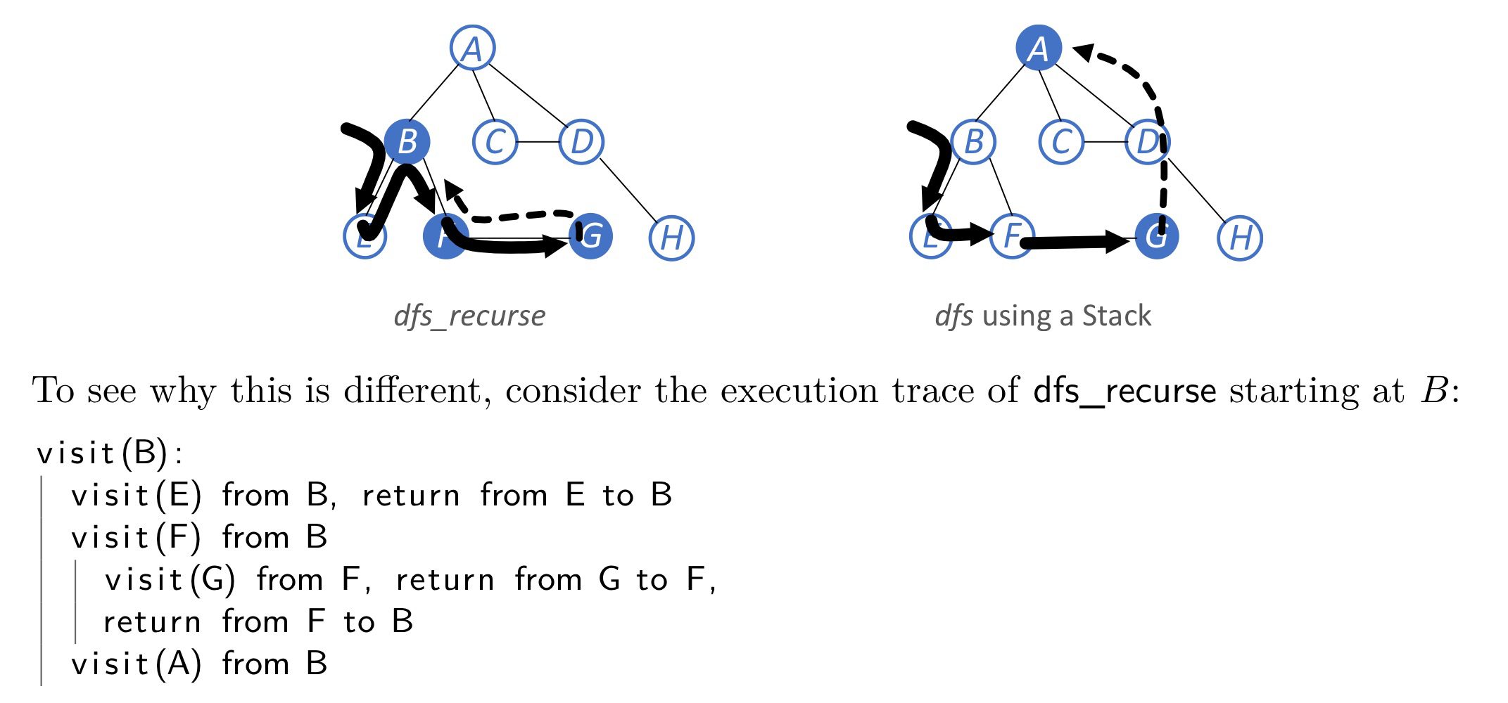
Depth-first search
Implementation 1: Recursion
Implementation 2: With a stack
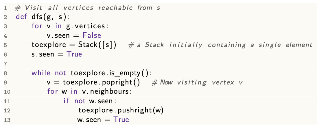
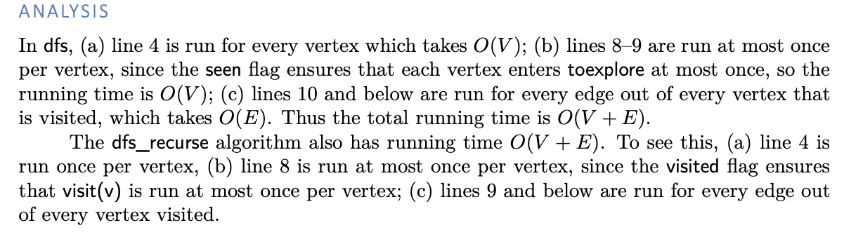
Analysis
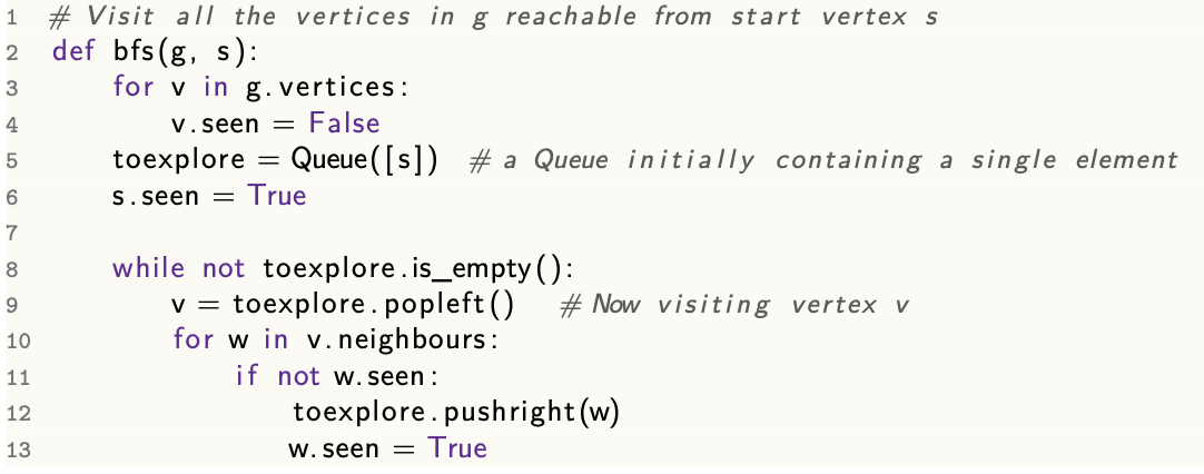
Breadth-first search
queue implementation
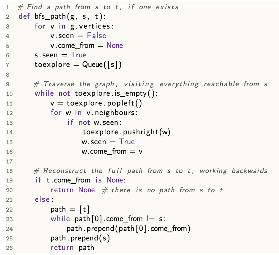
bfs_path
Dijkstra
Implementation
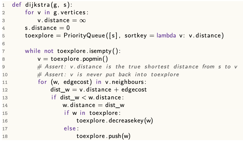
Analysis
Running time
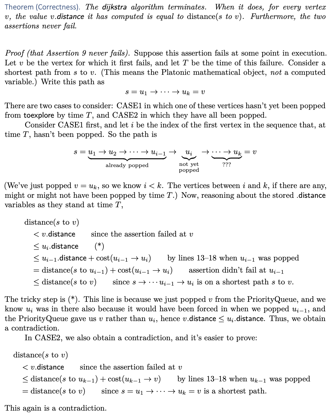
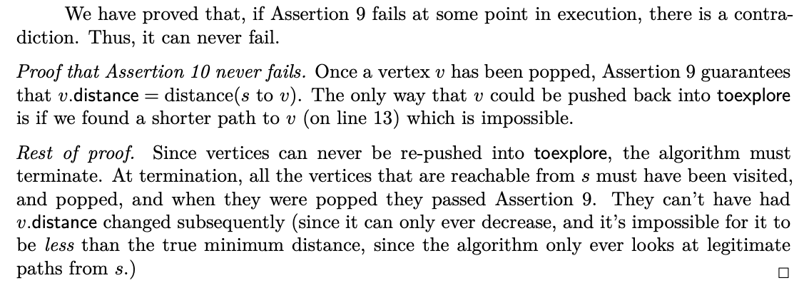
Correctness
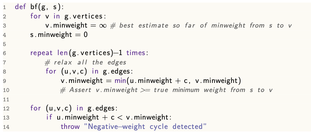
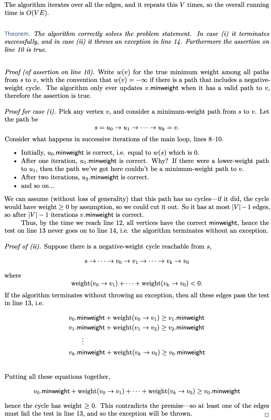
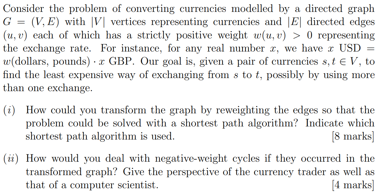
Bellman-Ford
Implementation
Analysis
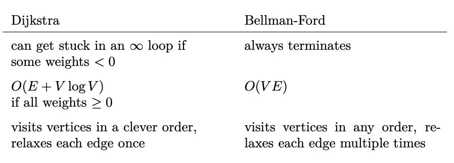
What are the advantages and disadvantages of the Bellman-Ford Algorithm in comparison to Dijkstra’s Algorithm?
Firstly, it can be applied to graphs with non-negative edges. Secondly, it can be also used to detect negative-weight cycles. The disadvantage of the Bellman-Ford Algorithm is the higher runtime which is O(VE), while Dijkstra’s Algorithm can be implemented in O(VlogV + E) time, which is much more efficient, especially if the given graph is sparse.
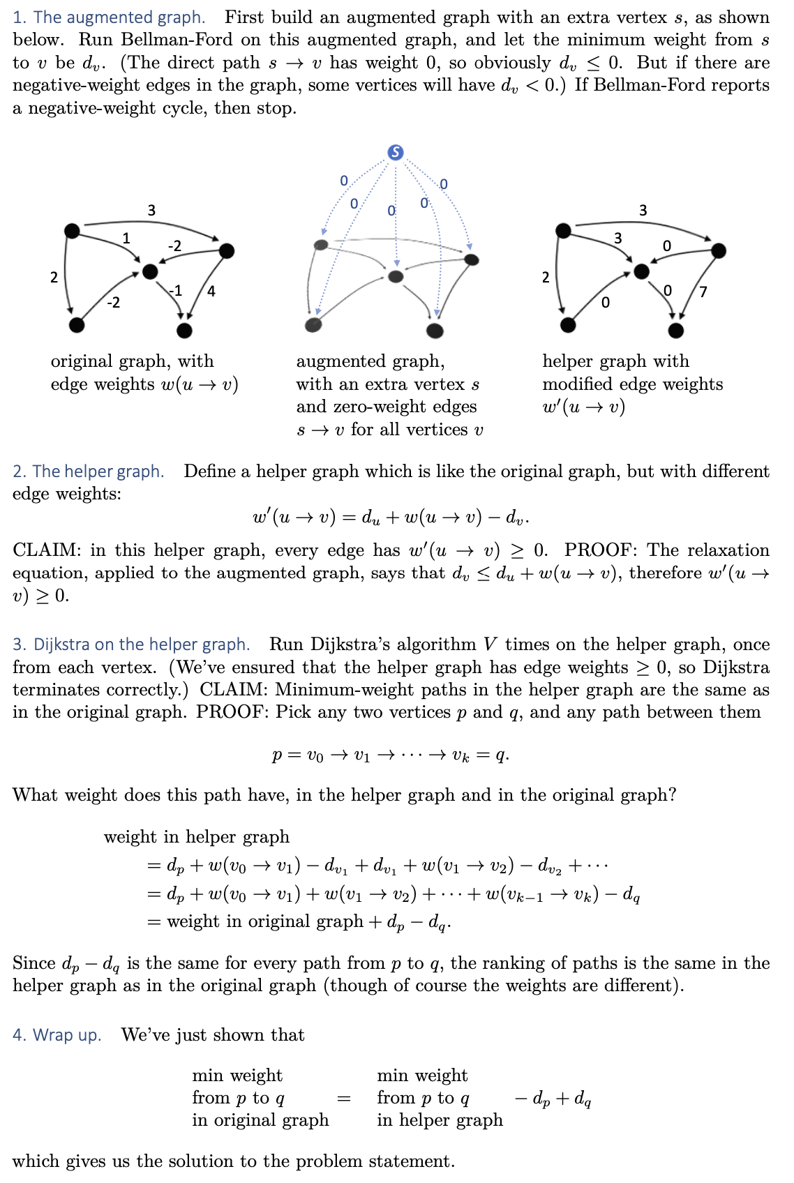
Johnson’s algorithm
Implementation
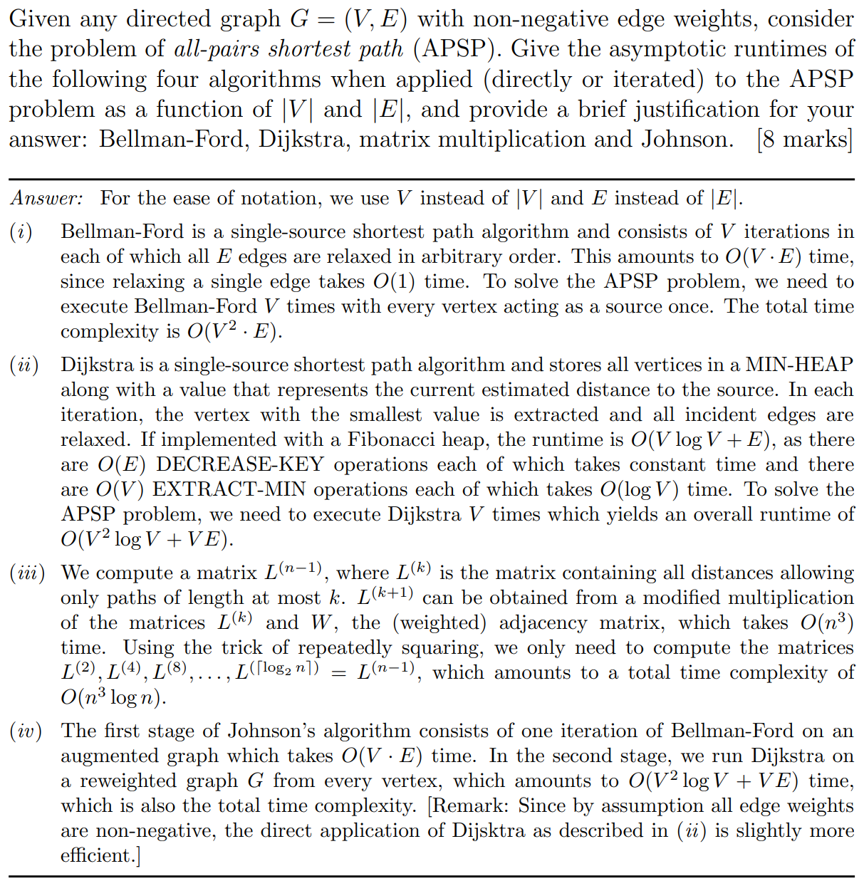
All-pair shortest path
All-pairs shortest path problem can be solved using the Floyd-Warshall algorithm or using repeated squaring in the adjacency matrix with modifications - which is a kind of a matrix multiplication.
Floyd-Warshall algorithm uses a dynamic programming approach to solve the all-pairs shortest path problem. Here’s a brief pseudocode for the algorithm:
1 | function FloydWarshall(graph) |
In the above pseudocode, graph is the adjacency matrix of the graph, and n is the number of vertices. The algorithm iteratively updates the shortest path between every pair of vertices (i, j) considering vertex k as an intermediate vertex. The final matrix dist contains the shortest path distances between every pair of vertices.
However, there is another method using repeated squaring of the adjacency matrix. If we multiply the adjacency matrix A by itself we get a new matrix A^2, where each element A^2[i][j] is the number of paths of length 2 from vertex i to vertex j. By taking higher powers of A, we can find the number of paths of any length. To find the shortest paths, we need to modify this slightly to keep track of the shortest path found so far. However, this method is more complex and generally not as efficient as Floyd-Warshall or Dijkstra’s algorithm for sparse graphs.
Past papers
What are the advantages and disadvantages of the Bellman-Ford Algorithm in comparison to Dijkstra’s Algorithm?
Firstly, it can be applied to graphs with non-negative edges [1 mark]. Secondly, it can be also used to detect negative-weight cycles [1 mark]. The disadvantage of the Bellman-Ford Algorithm is the higher runtime which is O(V · E), while Dijkstra’s Algorithm can be implemented in O(V log V + E) time, which is much more efficient, especially if the given graph is sparse
2014-p01-q10
Graphs and subgraphs
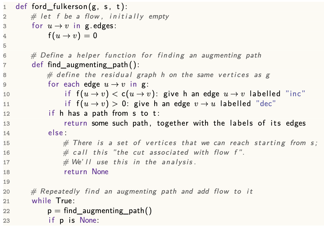
Ford-Fulkerson algorithm
Flow
A flow is a set of edge labels $f(u\rarr v)$ such that
$$
0 \le f(u\rarr v)\le c(u\rarr v) \text{ on every edge}
$$
$$
\text{value}(f) = \sum_{u:s\rarr u}f(s\rarr u)-\sum_{u:u\rarr s}f(u\rarr s)
$$
Flow Conservation
$$
\sum_{u:u\rarr v}f(u\rarr v)-\sum_{u:v\rarr u}f(v\rarr u)=0
$$
Implementation
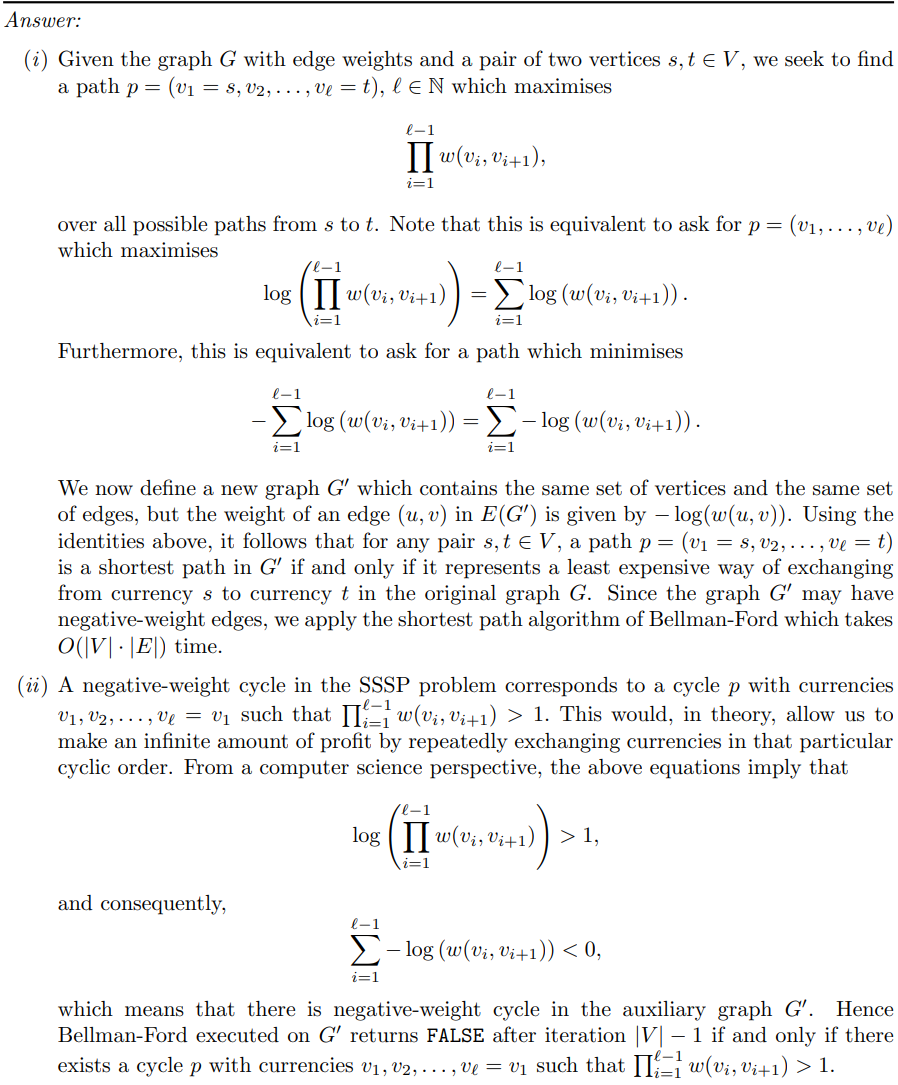
The residual graph
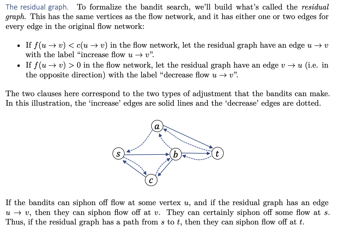
Augmenting paths
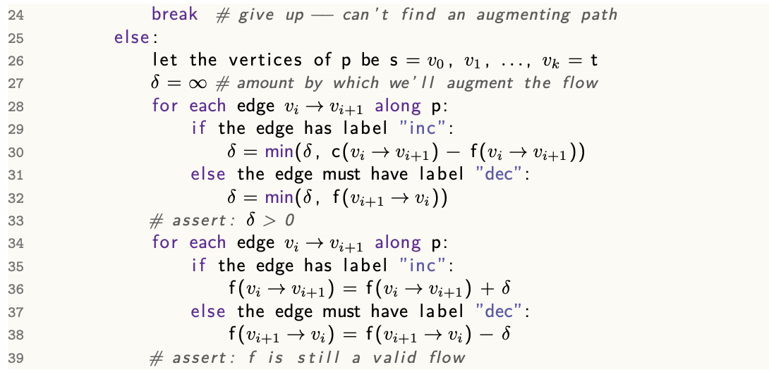
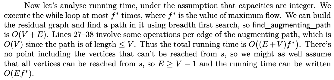
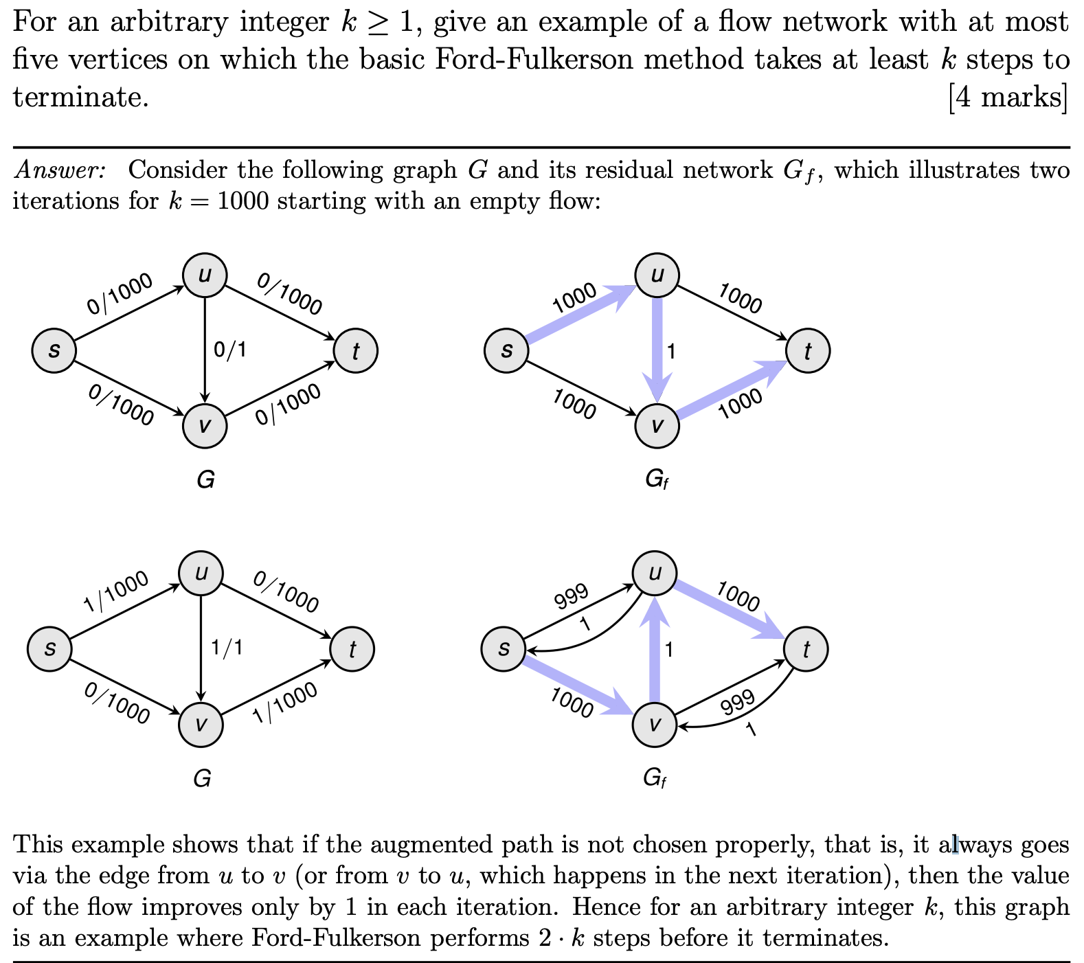
Analysis
Running time
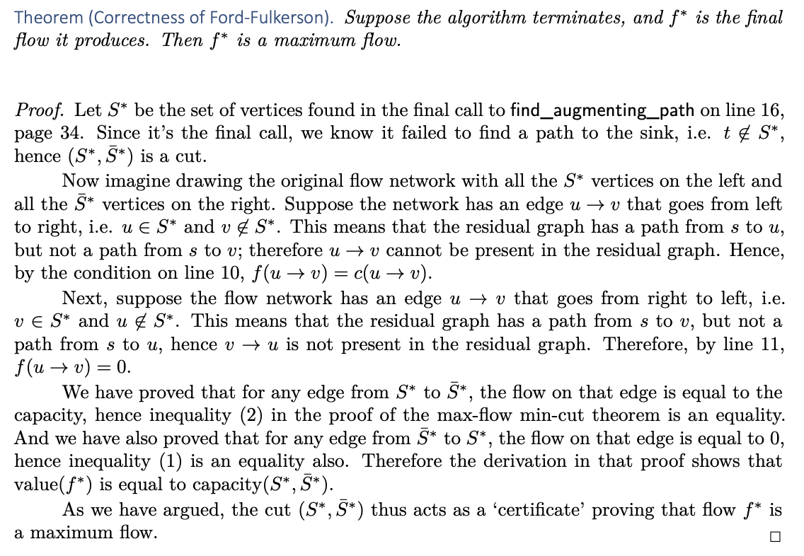
Correctness
Max-flow min-cut theorem
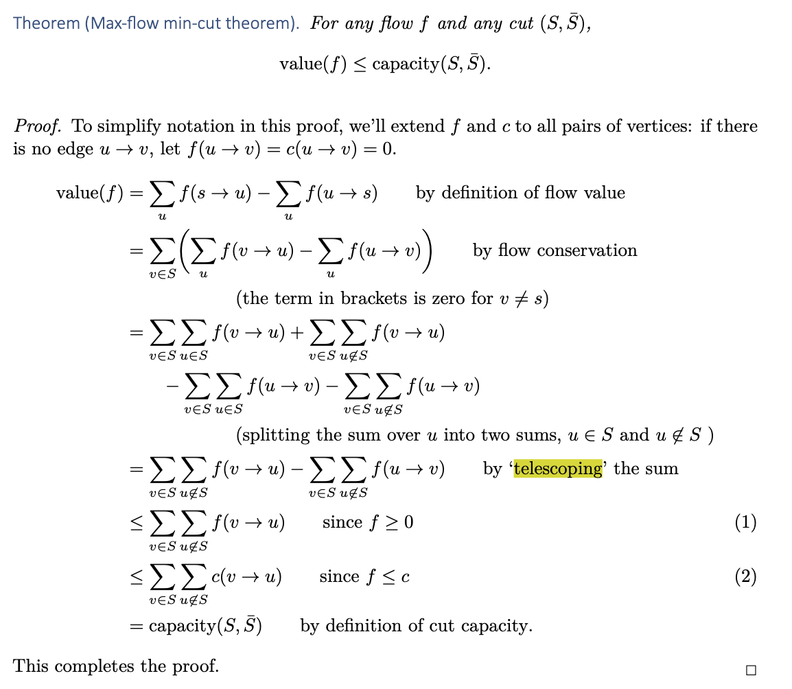
State the Max-Flow Min-Cut Theorem
For any flow network with source s and sink t, the value of maximum flow equals the minimum capacity of an (s,t) cut.
Past papers
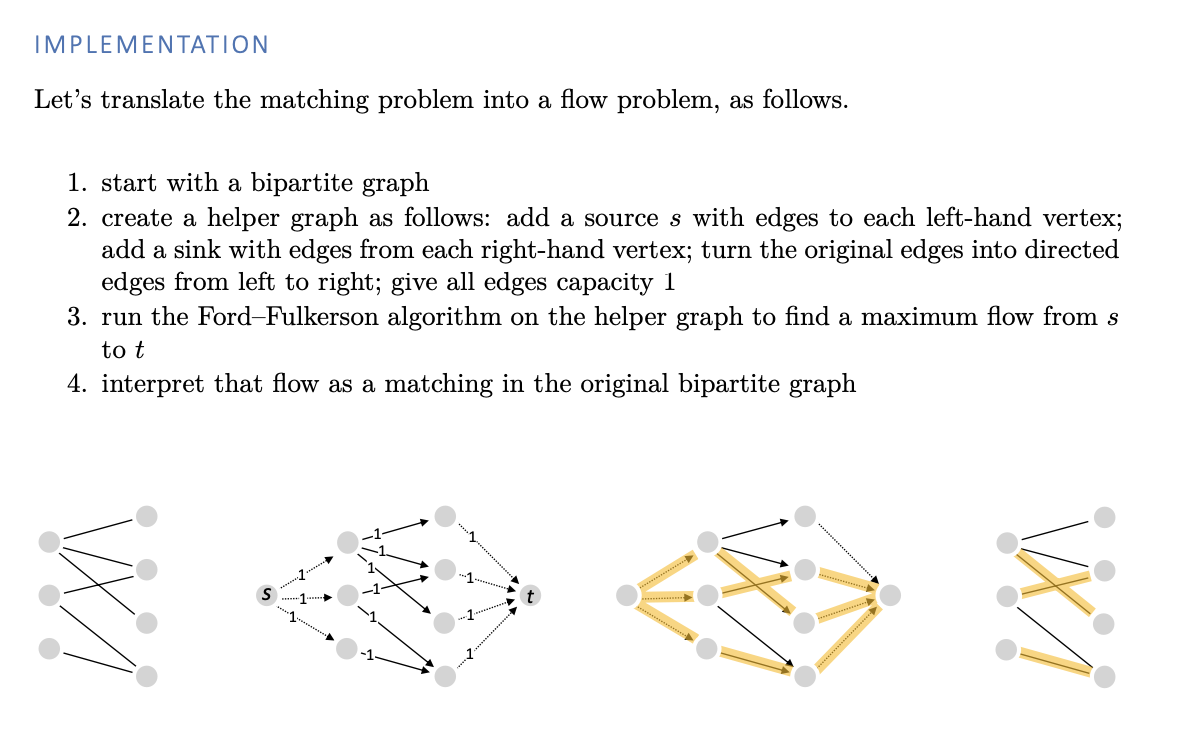
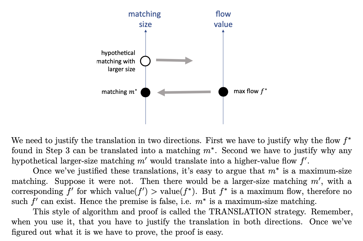
Matchings
Prim’s algorithm
Implementation
Analysis
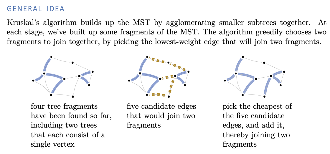
Kruskal’s algorithm
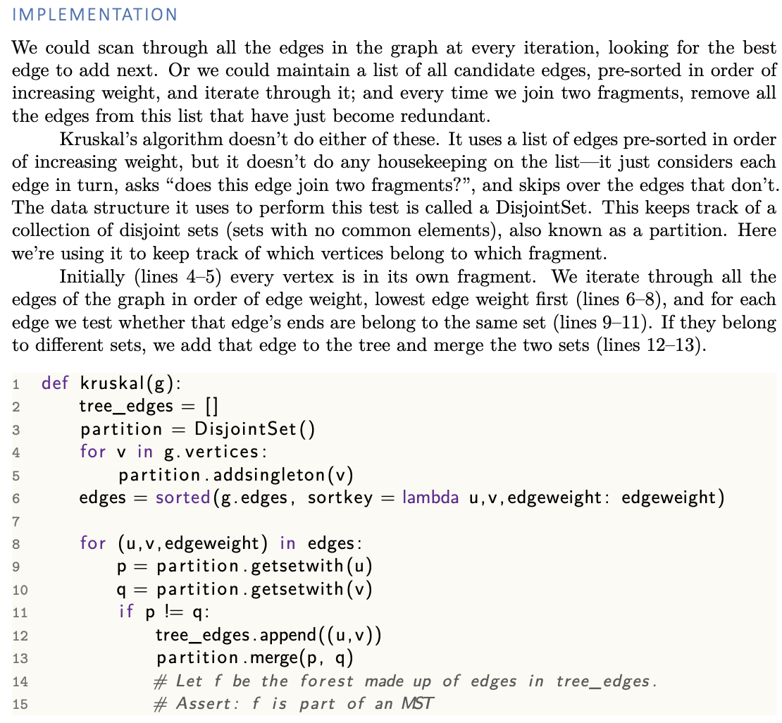
Implementation

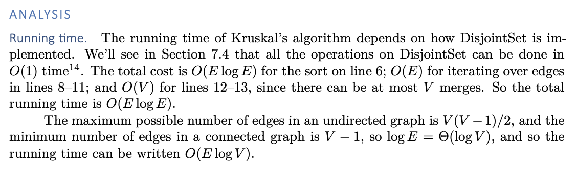
Analysis
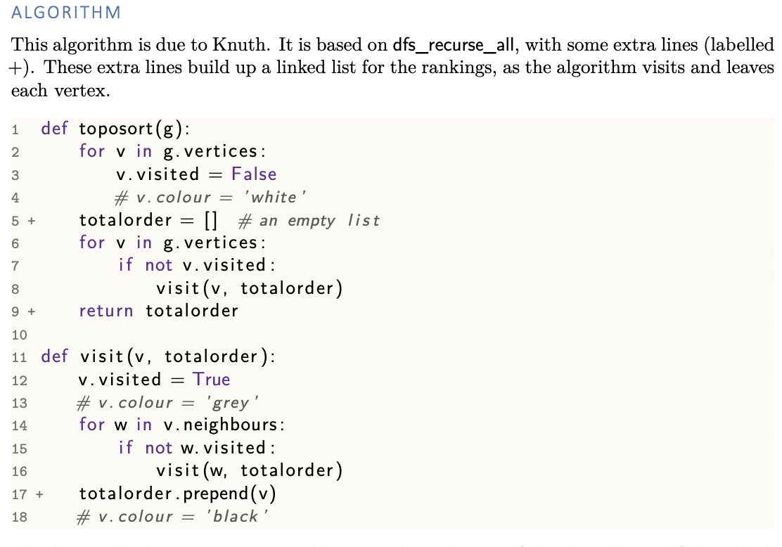
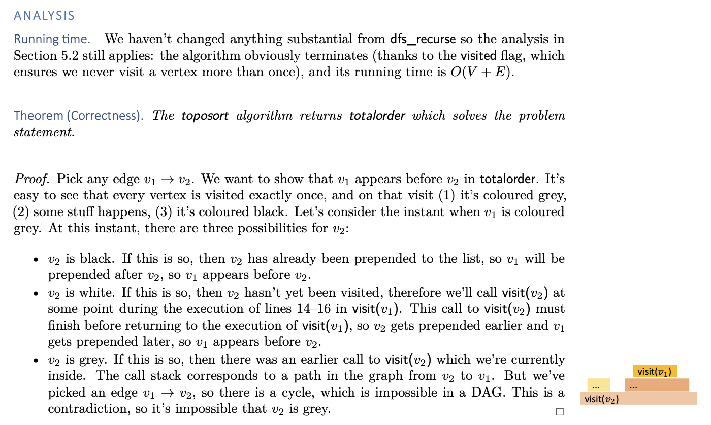
Topological sort
Analysis
Advanced data structures
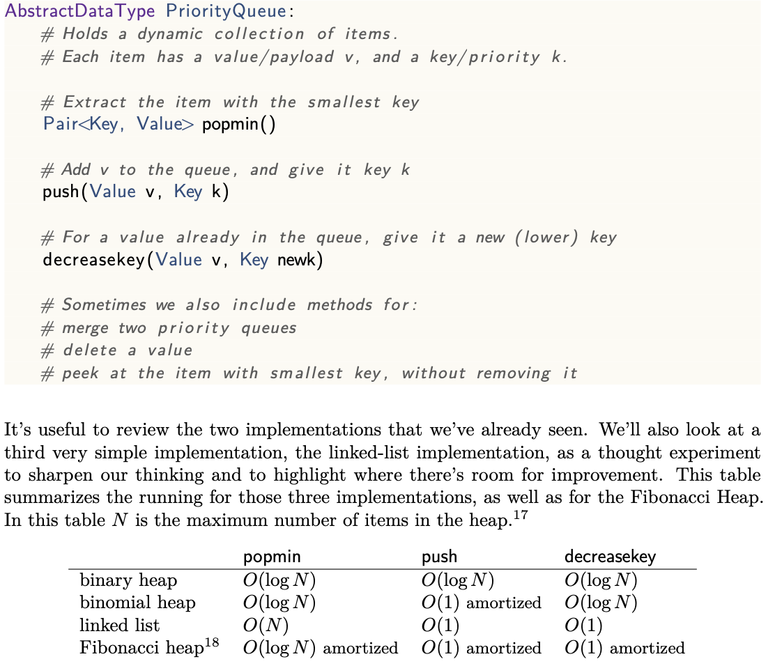
Priority queue
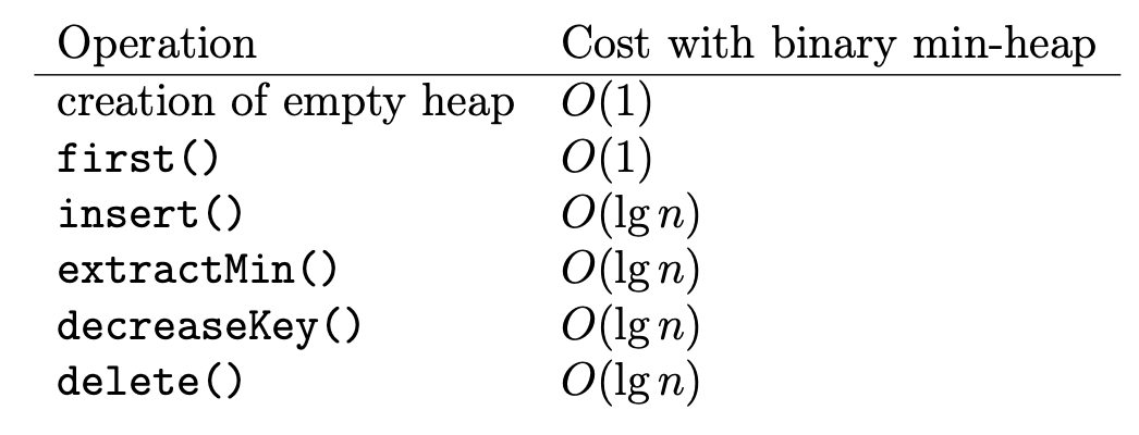
Binary heaps
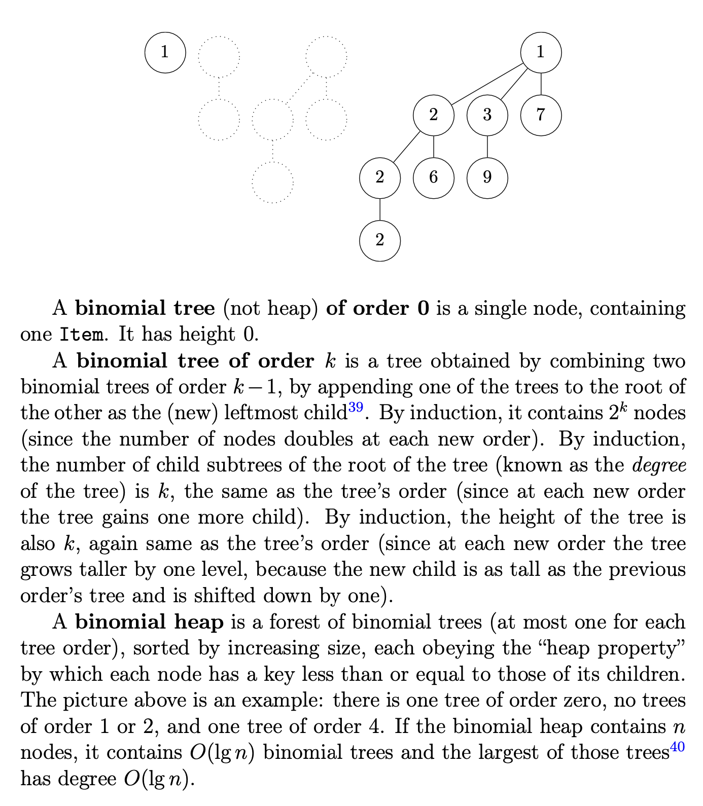
Binomial heaps
first()
To find the element with the smallest key in the whole binomial heap, scan the roots of all the binomial trees in the heap, at cost O(lg n) since there are that many trees.
extractMin()
To extract the element with the smallest key, which is necessarily a root, first find it, as above, at cost $O(lg n)$; then cut it out from its tree. Its children now form a forest of binomial trees of smaller orders, already sorted by decreasing size. Reverse this list of trees and you have another binomial heap. Merge this heap with what remains of the original one. Since the merge operation itself (q.v.) costs $O(lg n)$, this is also the total cost of extracting the minimum.
merge()
To merge two binomial heaps, examine their trees by increasing tree order and combine them following a procedure similar to the one used during binary addition with carry with a chain of full adders.
insert()
To insert a new element, consider it as a binomial heap with only one tree with only one node and merge it as above, at cost $O(lg n).$
decreaseKey()
To decrease the key of an item, proceed as in the case of a normal binary heap within the binomial tree to which the item belongs, at cost no greater than $O(lg n)$ which bounds the height of that tree.
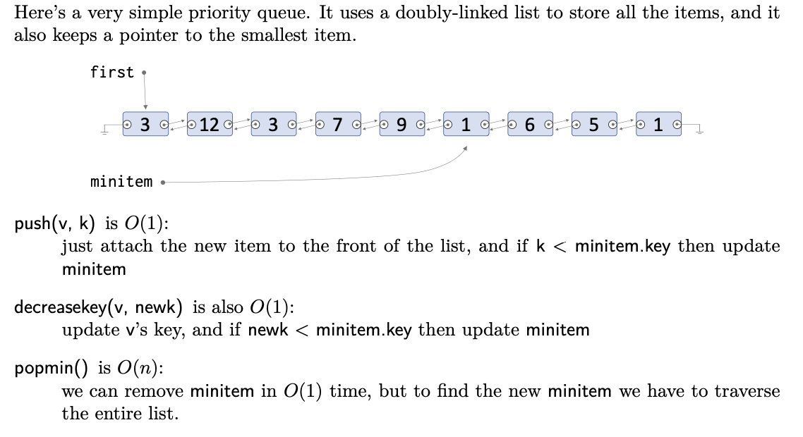
Linked List
Fibonacci heap
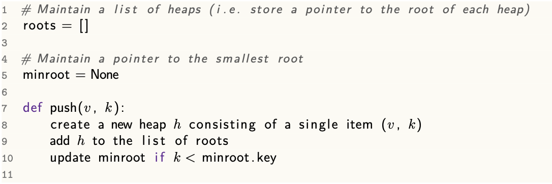
push()
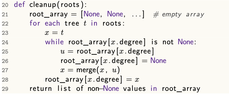
popmin()
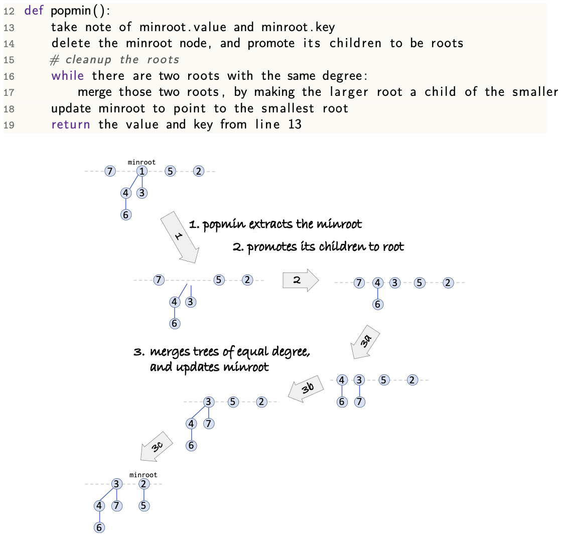
cleanup()
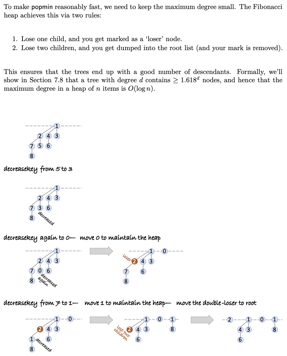
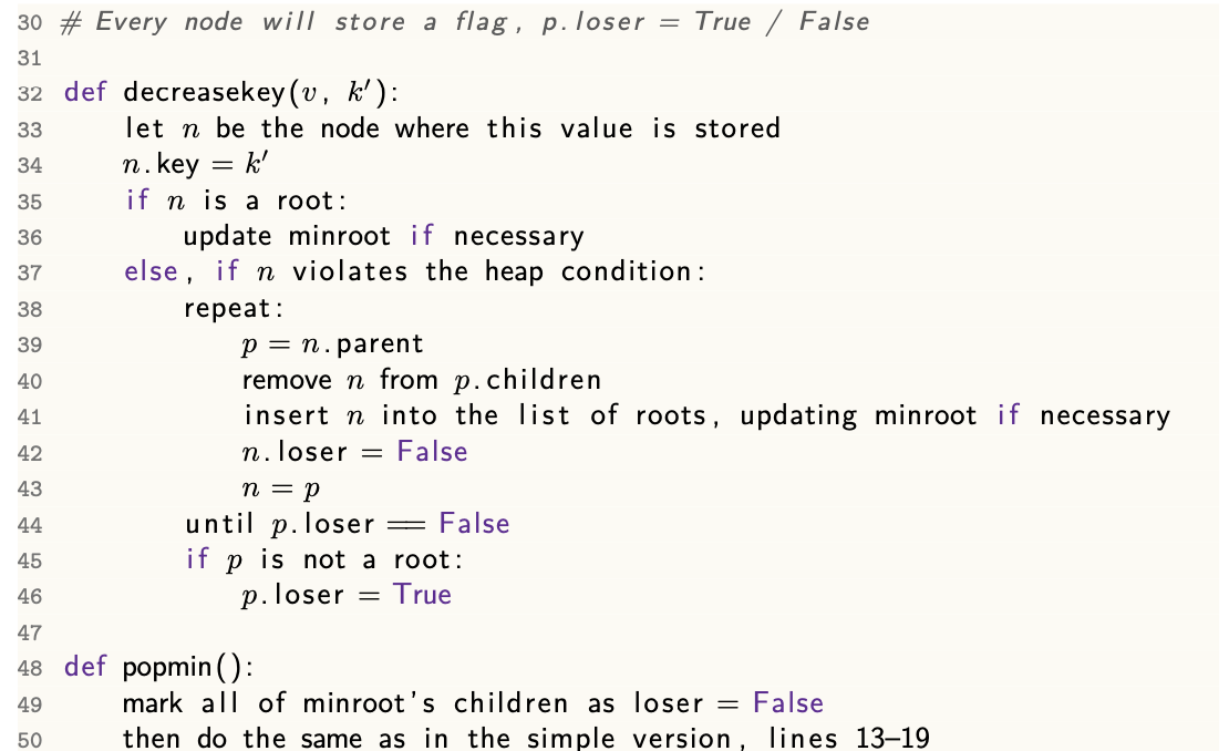
decrease key()
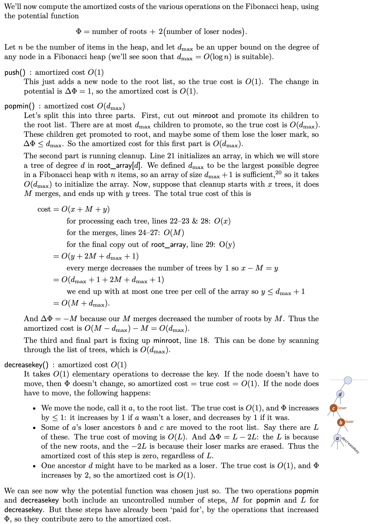
Analysis
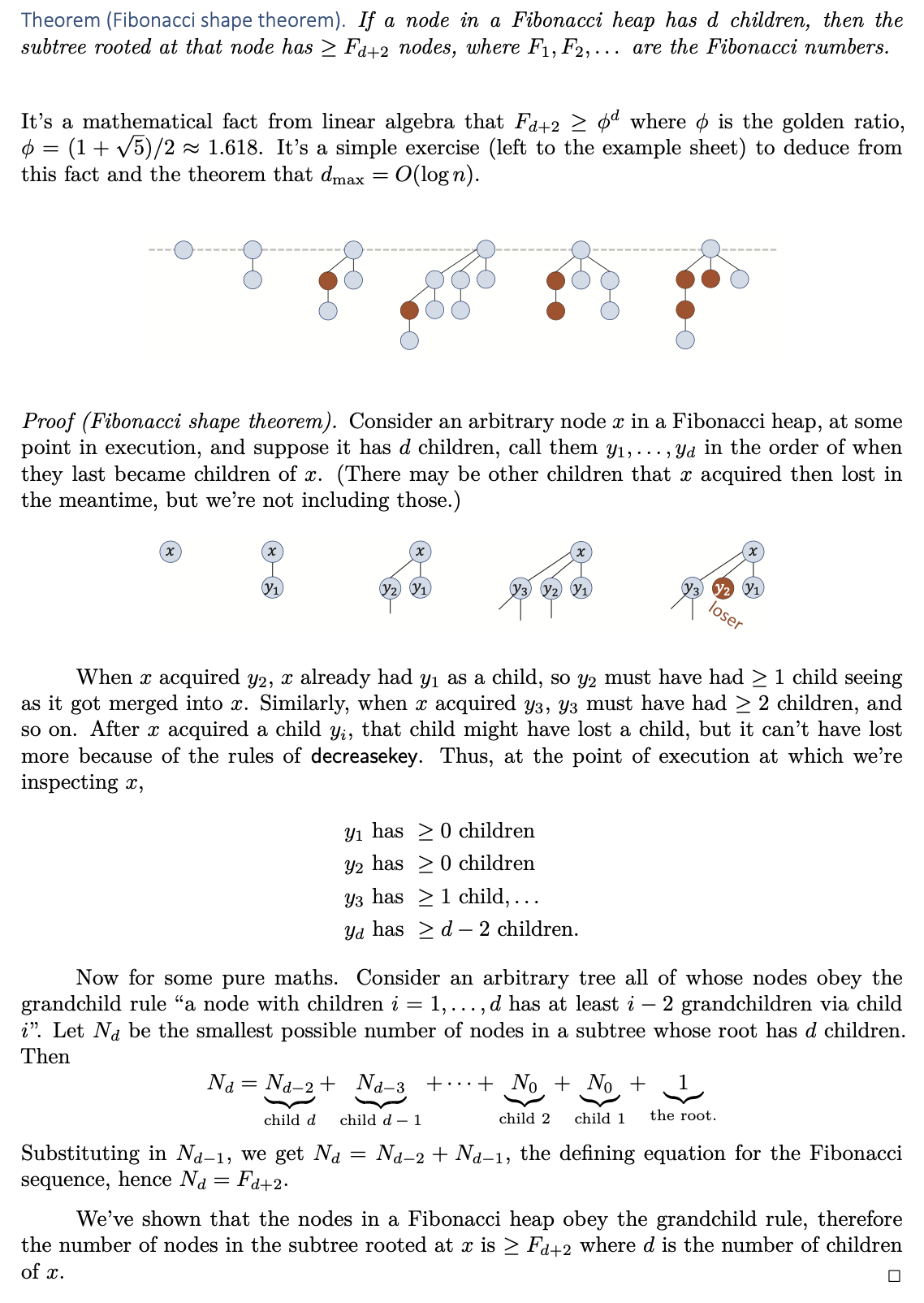
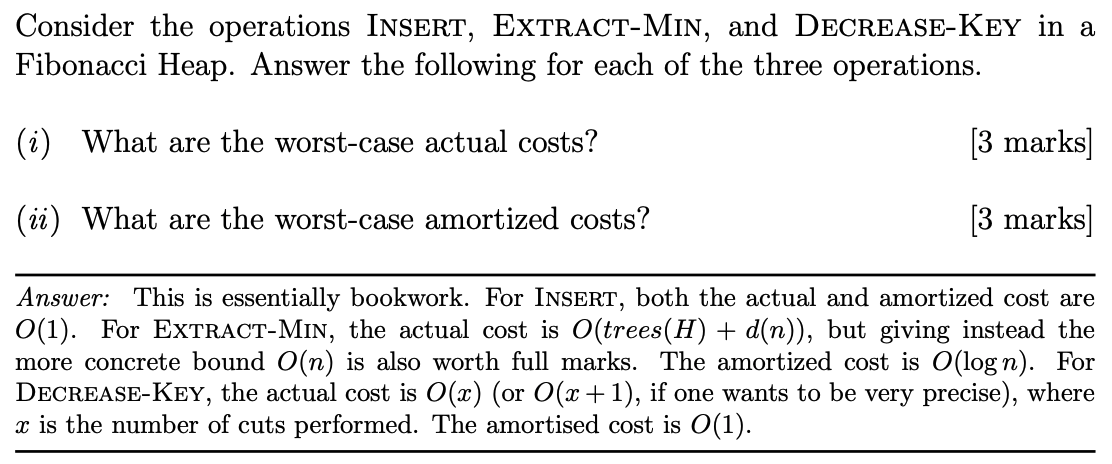
Fibonacci Shape Theorem
Past papers
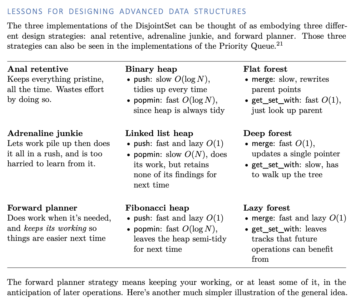
Disjoint set
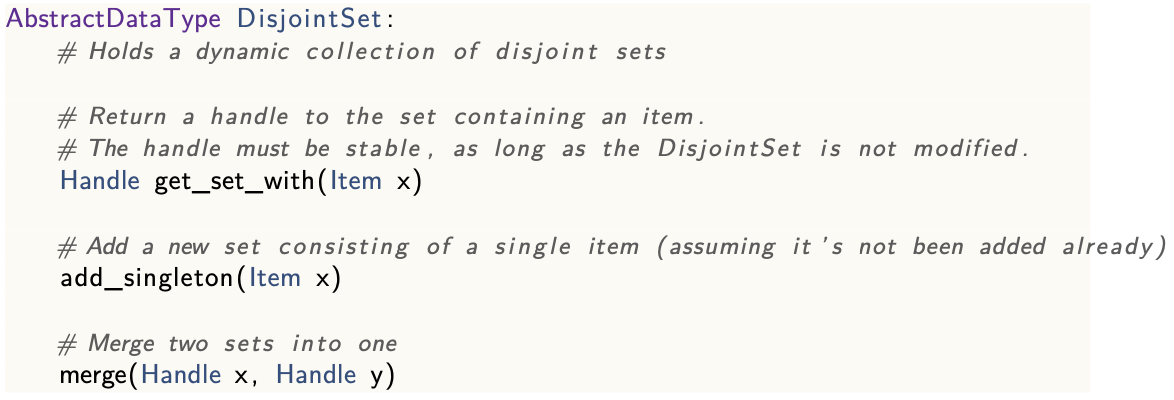
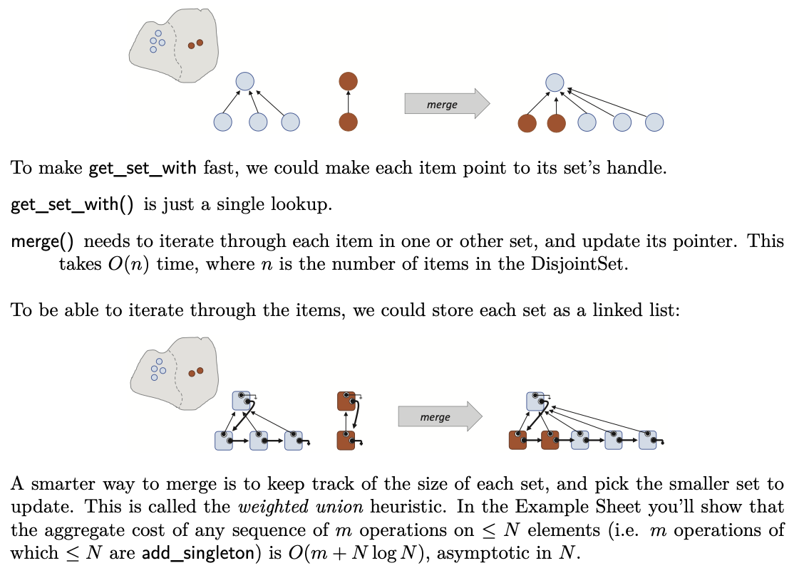
In a disjoint set, the weighted union heuristic says: keep track of the size of each set, and when you have to merge two sets then use the size information to decide which set to update, to reduce the amount of work. [Must include: keep track of the sizes.
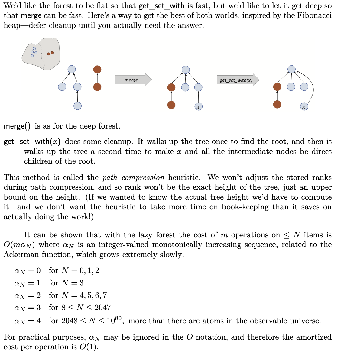
The path compression heuristic says: when you do a search, by following up a search tree to the root, then rewire the tree so that subsequent searches for the same element can be done quicker
Implementation1: Flat Forest
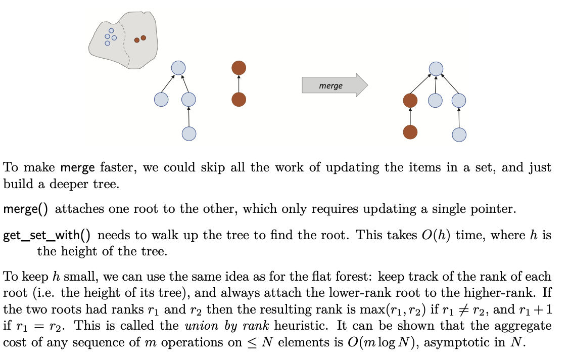
Implementation2: Deep Forest
Implementation3: Lazy Forest